ggtree v4.3.0 Learn more at https://yulab-smu.top/contribution-tree-data/

Please cite:

Guangchuang Yu, David Smith, Huachen Zhu, Yi Guan, Tommy Tsan-Yuk Lam.
ggtree: an R package for visualization and annotation of phylogenetic
trees with their covariates and other associated data. Methods in
Ecology and Evolution. 2017, 8(1):28-36. doi:10.1111/2041-210X.12628
Attaching package: 'ggtree'
The following object is masked from 'package:ape':

    rotate
The ggtree(Yu et al., 2017) supports many ways of manipulating the tree visually, including viewing selected clade to explore large tree (Figure Figure 7.1), taxa clustering (Figure Figure 7.6), rotating clade or tree (Figure Figure 7.7 (b) and Figure 7.9), zoom out or collapsing clades (Figure Figure 7.3 (a) and Figure 7.2), etc.. Details of the tree manipulation functions are summarized in Table Table 7.1.
Table 7.1: Tree manipulation functions.
Function
Description
collapse
Collapse a selecting clade
expand
Expand collapsed clade
flip
Exchange position of 2 clades that share a parent node
groupClade
Grouping clades
groupOTU
Grouping OTUs by tracing back to the most recent common ancestor
identify
Interactive tree manipulation
rotate
Rotating a selected clade by 180 degrees
rotate_tree
Rotating circular layout tree by a specific angle
scaleClade
Zoom in or zoom out selecting clade
open_tree
Convert a tree to fan layout by specific open angle
7.1 Viewing Selected Clade
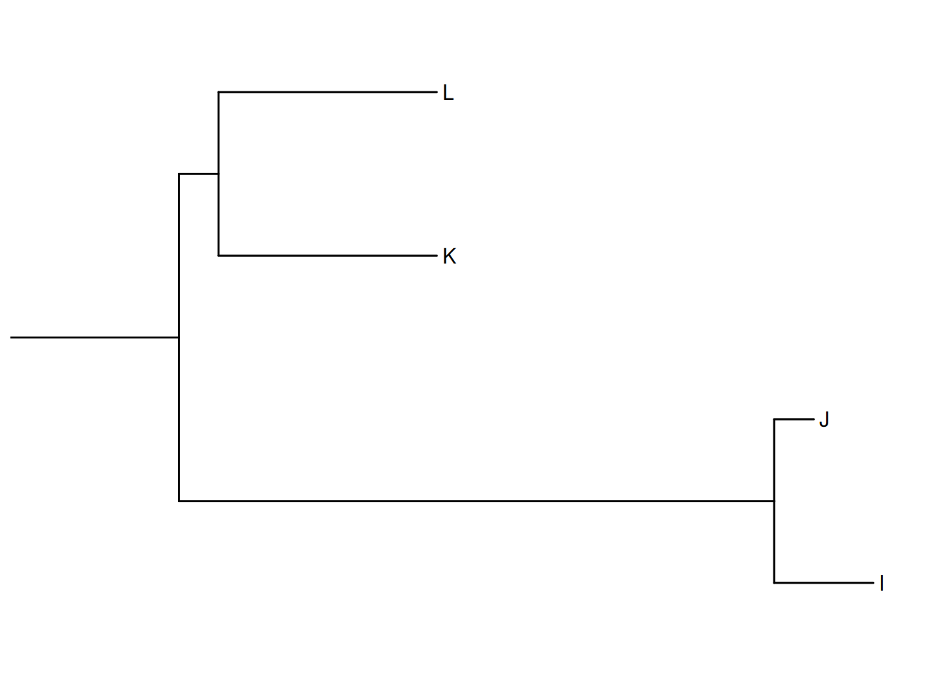
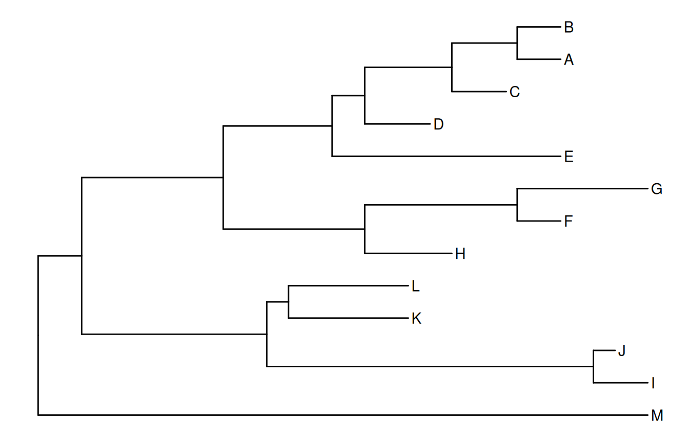
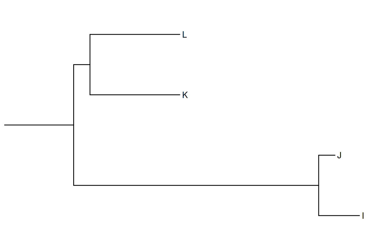
A clade is a monophyletic group that contains a single ancestor and all of its descendants. We can visualize a specifically selected clade via the viewClade() function as demonstrated in Figure Figure 7.1 (b). Another solution is to extract the selected clade as a new tree object as described in session 2.5. These functions are developed to help users explore a large tree.
Viewing a selected clade of a tree. An example tree used to demonstrate how r Biocpkg("ggtree") supports exploring or manipulating phylogenetic tree visually (A). The r Biocpkg("ggtree") supports visualizing selected clade (B). A clade can be selected by specifying a node number or determined by the most recent common ancestor of selected tips.
(a) Example tree used to demonstrate visual exploration
(b) Visualizing a selected clade
Figure 7.1: Viewing a selected clade of a tree.
Some of the functions, e.g., viewClade(), work with clade and accept a parameter of an internal node number. To get the internal node number, users can use the MRCA() function (as in Figure Figure 7.1) by providing two taxa names. The function will return the node number of input taxa’s most recent common ancestor (MRCA). It works with a tree and graphic (i.e., the ggtree() output) object. The tidytree package also provides an MRCA() method to extract information from the MRCA node (see details in session 2.1.3).
7.2 Scaling Selected Clade
The ggtree provides another option to zoom out (or compress) selected clades via the scaleClade() function. In this way, we retain the topology and branch lengths of compressed clades. This helps to save the space to highlight those clades of primary interest in the study.
Figure 7.2: Scaling selected clade. Clades can be zoomed in (if scale > 1) to highlight or zoomed out to save space.
If users want to emphasize important clades, they can use the scaleClade() function by passing a numeric value larger than 1 to the scale parameter. Then the selected clade will be zoomed in. Users can also use the groupClade() function to assign selected clades with different clade IDs which can be used to color these clades with different colors as shown in Figure Figure 7.2.
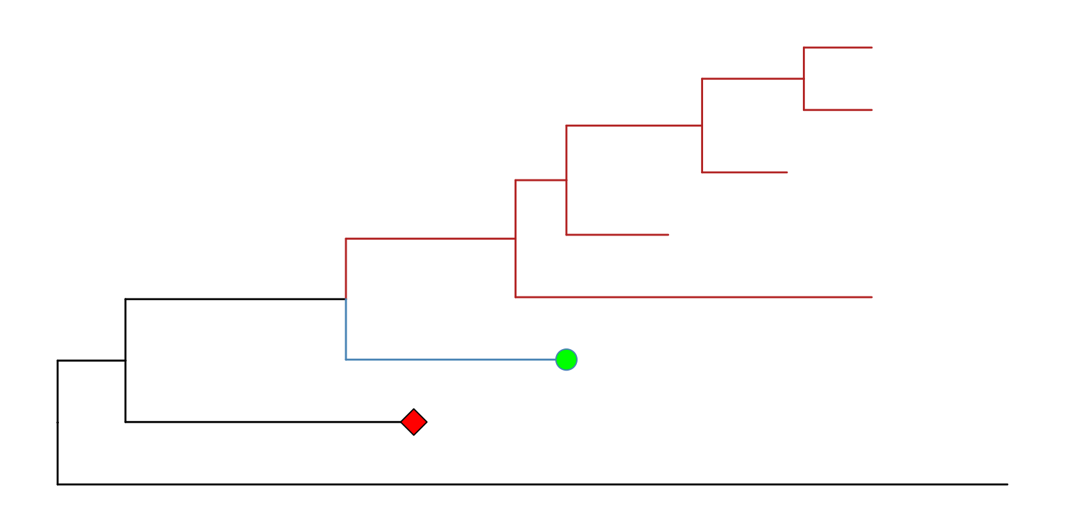
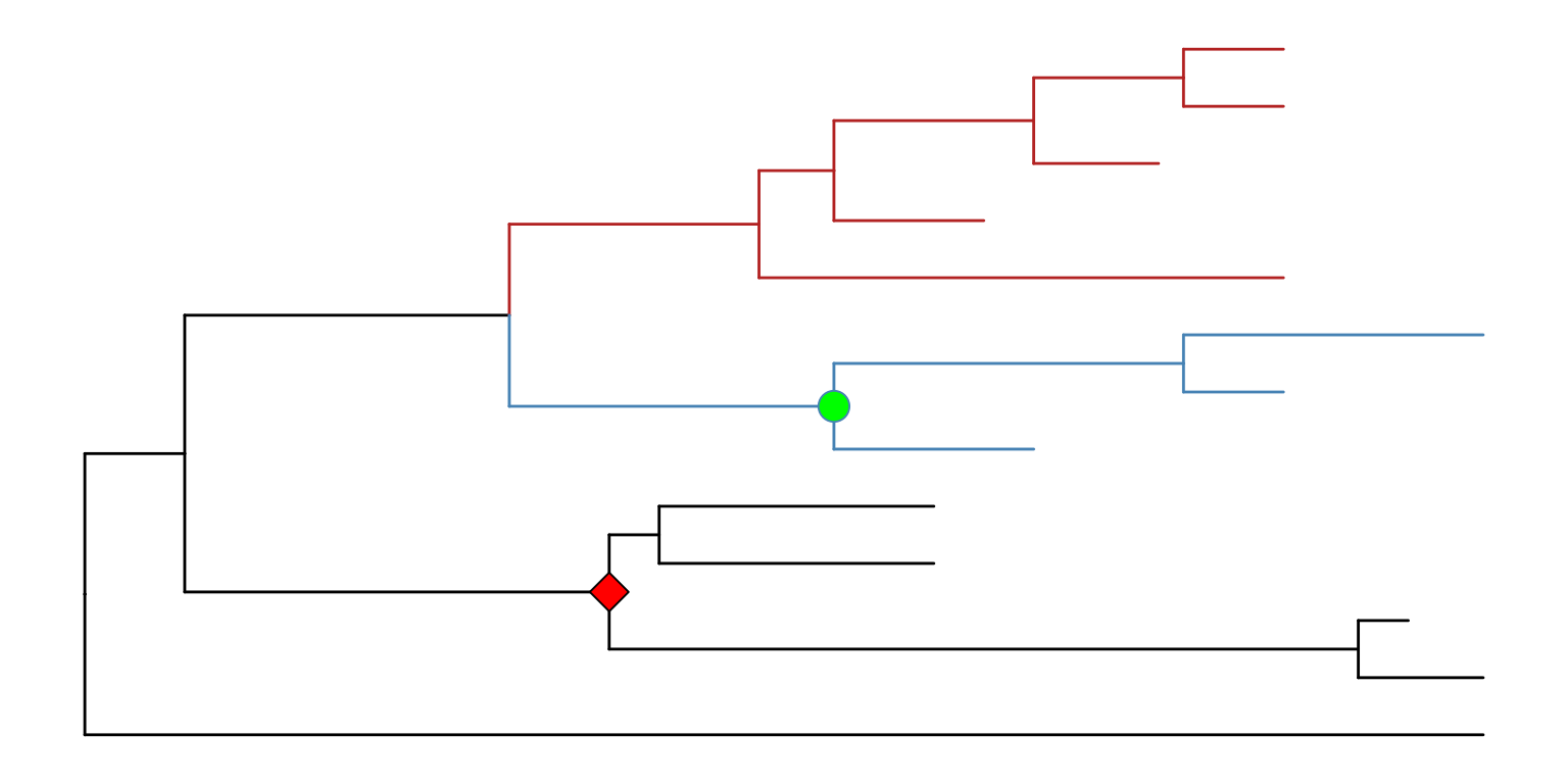
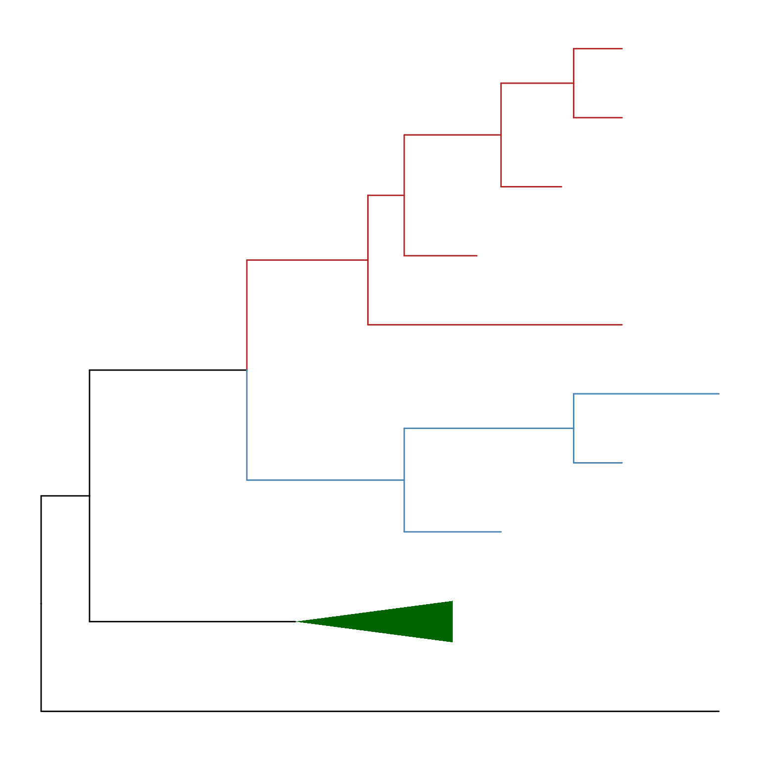
7.3 Collapsing and Expanding Clade
It is a common practice to prune or collapse clades so that certain aspects of a tree can be emphasized. The ggtree supports collapsing selected clades using the collapse() function as shown in Figure Figure 7.3 (a).
Figure 7.3: Collapsing selected clades and expanding collapsed clades.
Here two clades were collapsed and labeled by the green circle and red square symbolic points. Collapsing is a common strategy to collapse clades that are too large for displaying in full or are not the primary interest of the study. In ggtree, we can expand (i.e., uncollapse) the collapsed branches back with the expand() function to show details of species relationships as demonstrated in Figure Figure 7.3 (b).
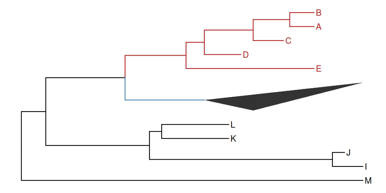
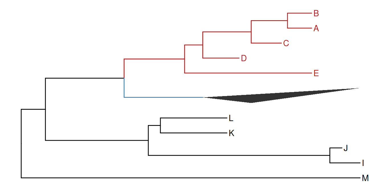
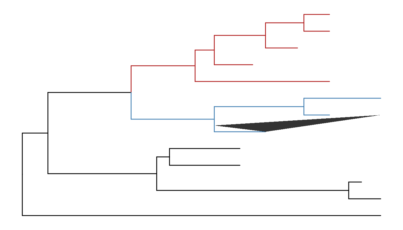
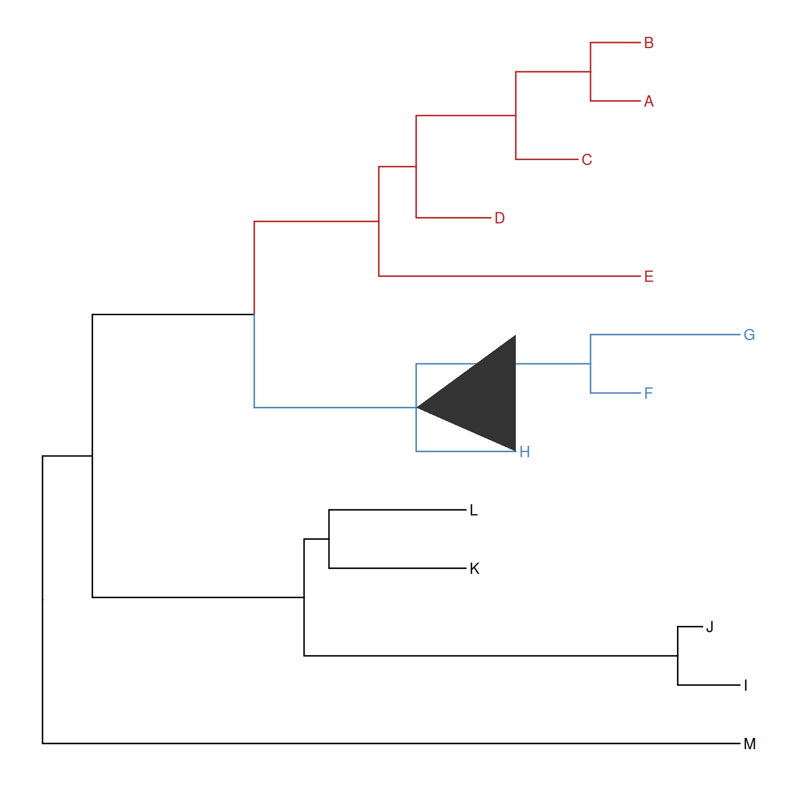
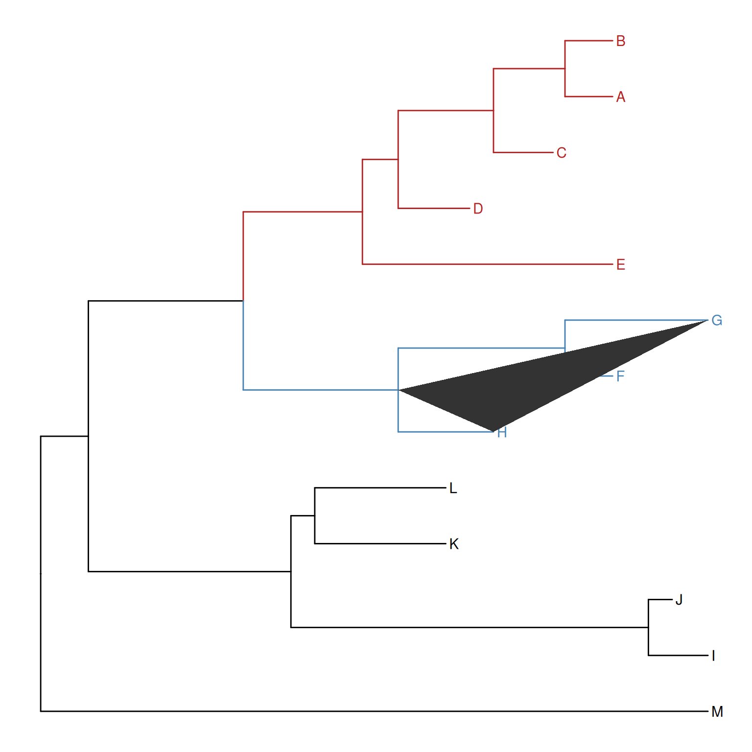
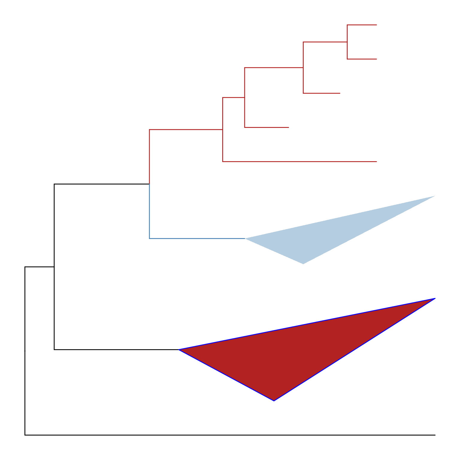
Triangles are often used to represent the collapsed clade and ggtree also supports it. The collapse() function provides a mode parameter, which by default is "none" and the selected clade is collapsed as a tip. Users can specify the mode to "max" that uses the farthest tip (Figure Figure 7.5 (a)), "min" that uses the closest tip (Figure Figure 7.5 (b)), and "mixed" that uses both (Figure Figure 7.5 (c)).
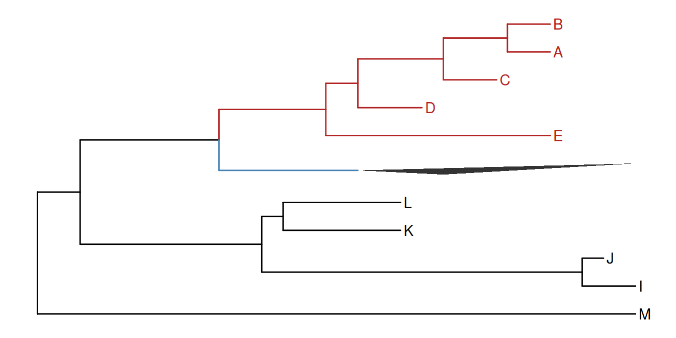
The height parameter can be used to control the displayed height of collapsed triangles. It supports three input forms: NULL (default, keep the original triangle height), ggplot2::rel() to scale the original triangle height relatively, and a numeric value to force an absolute displayed height. This is useful when multiple collapsed clades should have a comparable visual footprint. After collapsing with a custom height, expand() restores the original layout correctly (Figure Figure 7.4).
The groupClade() function assigns the branches and nodes under different clades into different groups. It accepts an internal node or a vector of internal nodes to cluster clade/clades.
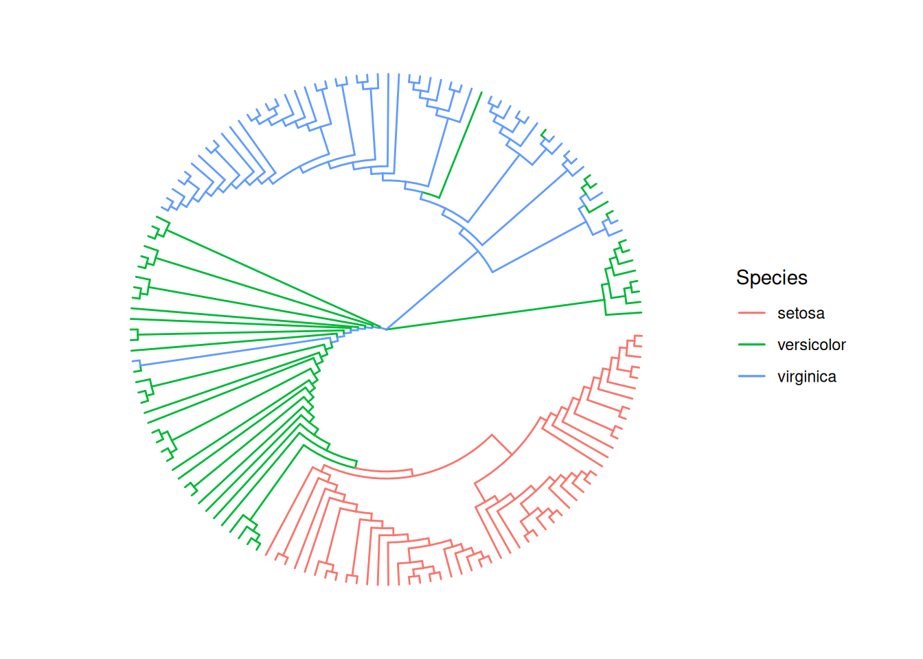
Similarly, the groupOTU() function assigns branches and nodes to different groups based on user-specified groups of operational taxonomic units (OTUs) that are not necessarily within a clade but can be monophyletic (clade), polyphyletic or paraphyletic. It accepts a vector of OTUs (taxa name) or a list of OTUs and will trace back from OTUs to their most recent common ancestor (MRCA) and cluster them together as demonstrated in Figure Figure 7.6.
A phylogenetic tree can be annotated by mapping different line types, sizes, colors, or shapes of the branches or nodes that have been assigned to different groups.
Figure 7.6: Grouping OTUs. OTU clustering based on their relationships. Selected OTUs and their ancestors up to the MRCA will be clustered together.
We can group taxa at the tree level. The following code will produce an identical figure of Figure Figure 7.6 (see more details described in session 2.2.3).
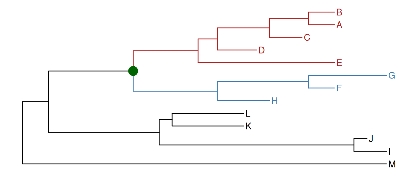
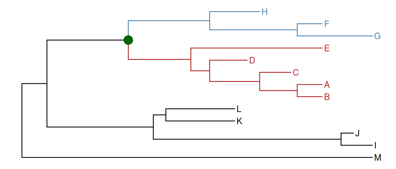
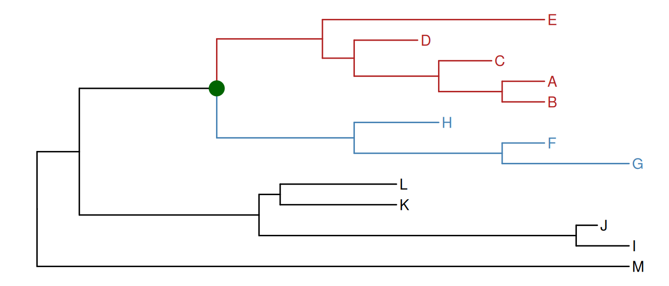
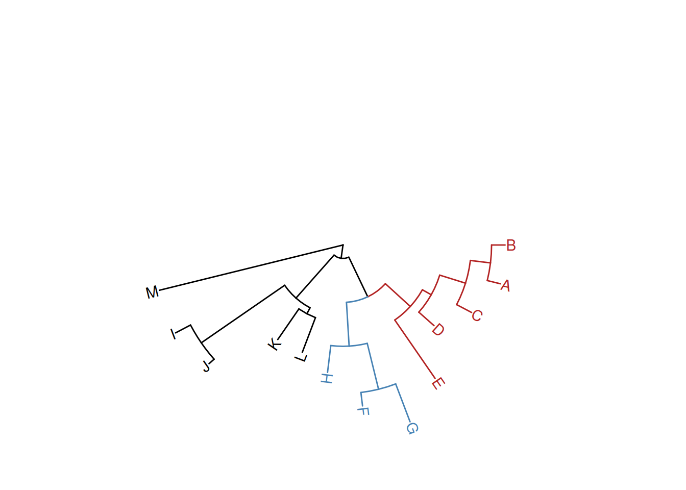
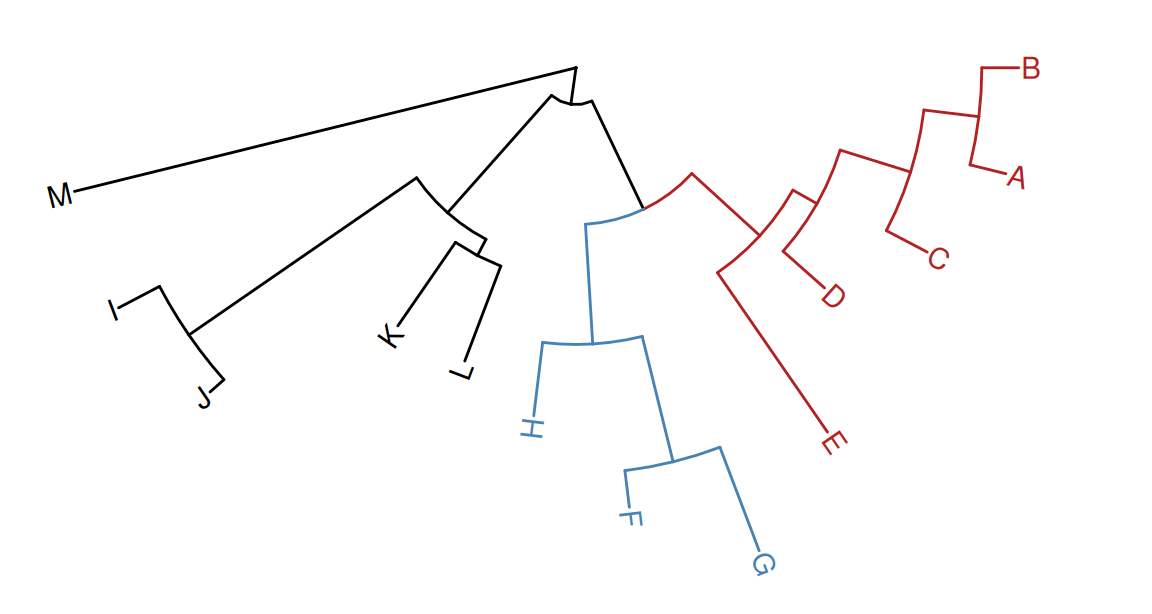
To facilitate exploring the tree structure, ggtree supports rotating selected clade by 180 degrees using the rotate() function (Figure Figure 7.7 (b)). Position of immediate descendant clades of the internal node can be exchanged via flip() function (Figure Figure 7.7 (c)).
p1 <- p +geom_point2(aes(subset=node==16), color='darkgreen', size=5)p2 <-rotate(p1, 16)flip(p2, 17, 21)
(a) Original tree with selected clade
(b) Rotate selected clade by 180 degrees
(c) Flip immediate descendant clades
Figure 7.7: Exploring tree structure. A clade (indicated by a dark green circle) in a tree (A) can be rotated by 180° (B) and the positions of its immediate descendant clades (colored by blue and red) can be exchanged (C).
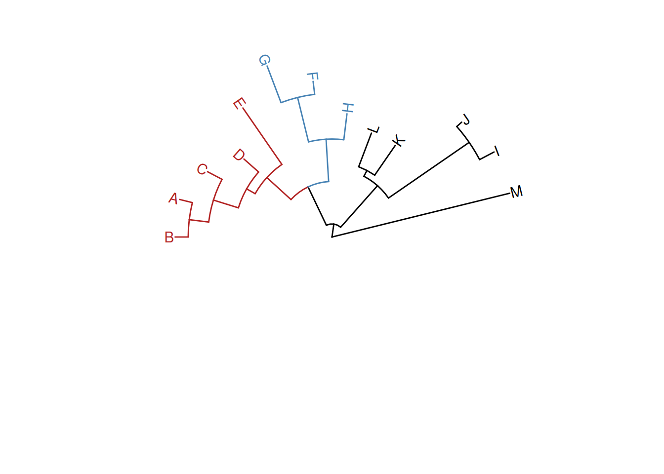
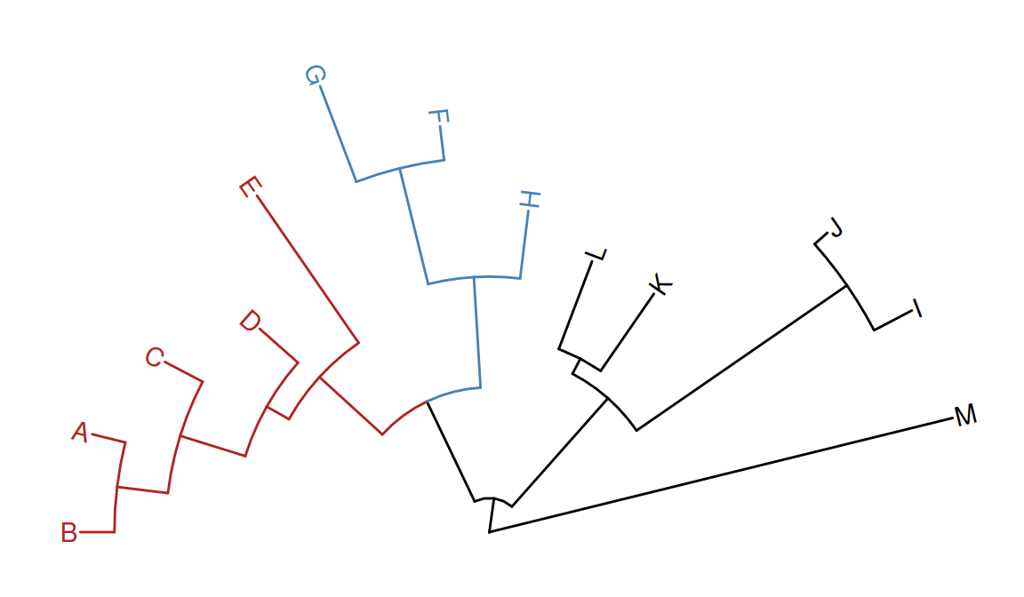
Most of the tree manipulation functions are working on clades, while ggtree also provides functions to manipulate a tree, including open_tree() to transform a tree in either rectangular or circular layout to the fan layout, and rotate_tree() function to rotate a tree for specific angle in both circular or fan layouts, as demonstrated in Figures Figure 7.8 and Figure 7.9.
p3 <-open_tree(p, 180) +geom_tiplab()
Scale for y is already present.
Adding another scale for y, which will replace the existing scale.
Scale for y is already present.
Adding another scale for y, which will replace the existing scale.
print(p3)
Scale for y is already present.
Adding another scale for y, which will replace the existing scale.
Scale for y is already present.
Adding another scale for y, which will replace the existing scale.
Figure 7.8: Transforming a tree to fan layout. A tree can be transformed to a fan layout by open_tree with a specific angle.
rotate_tree(p3, 180)
Coordinate system already present.
ℹ Adding new coordinate system, which will replace the existing one.
Coordinate system already present.
ℹ Adding new coordinate system, which will replace the existing one.
Figure 7.9: Rotating tree. A circular/fan layout tree can be rotated by any specific angle.
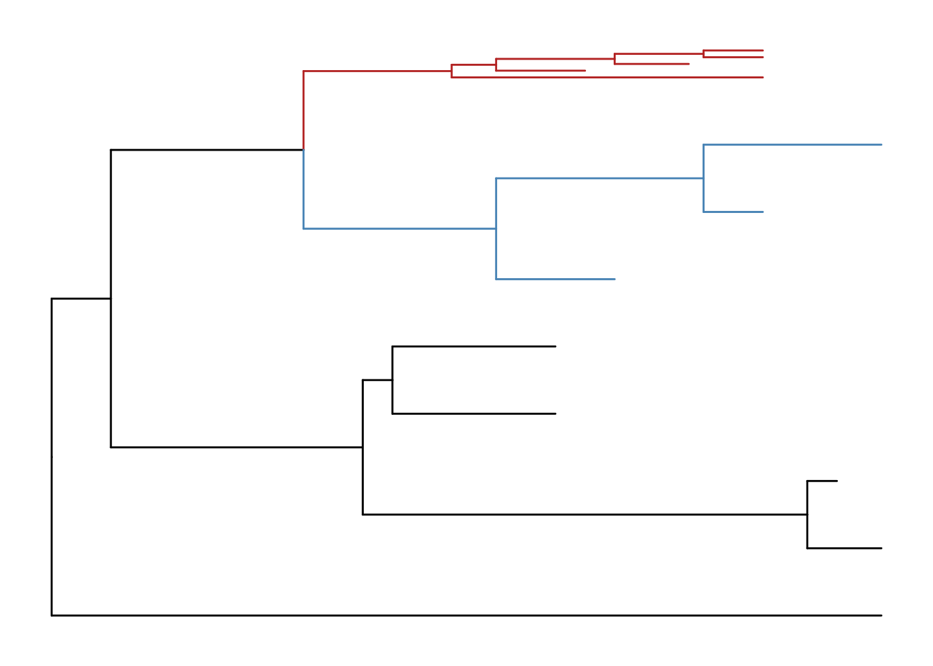
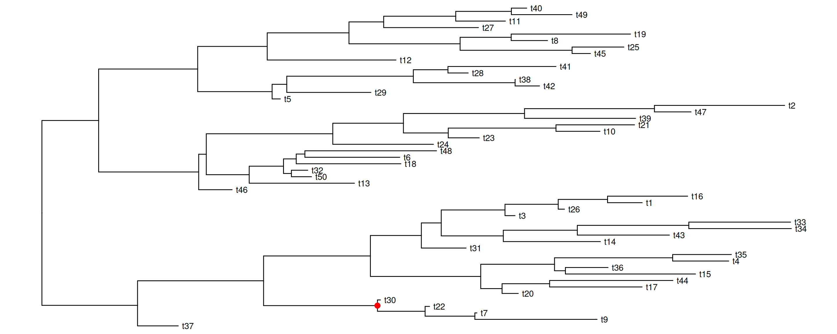
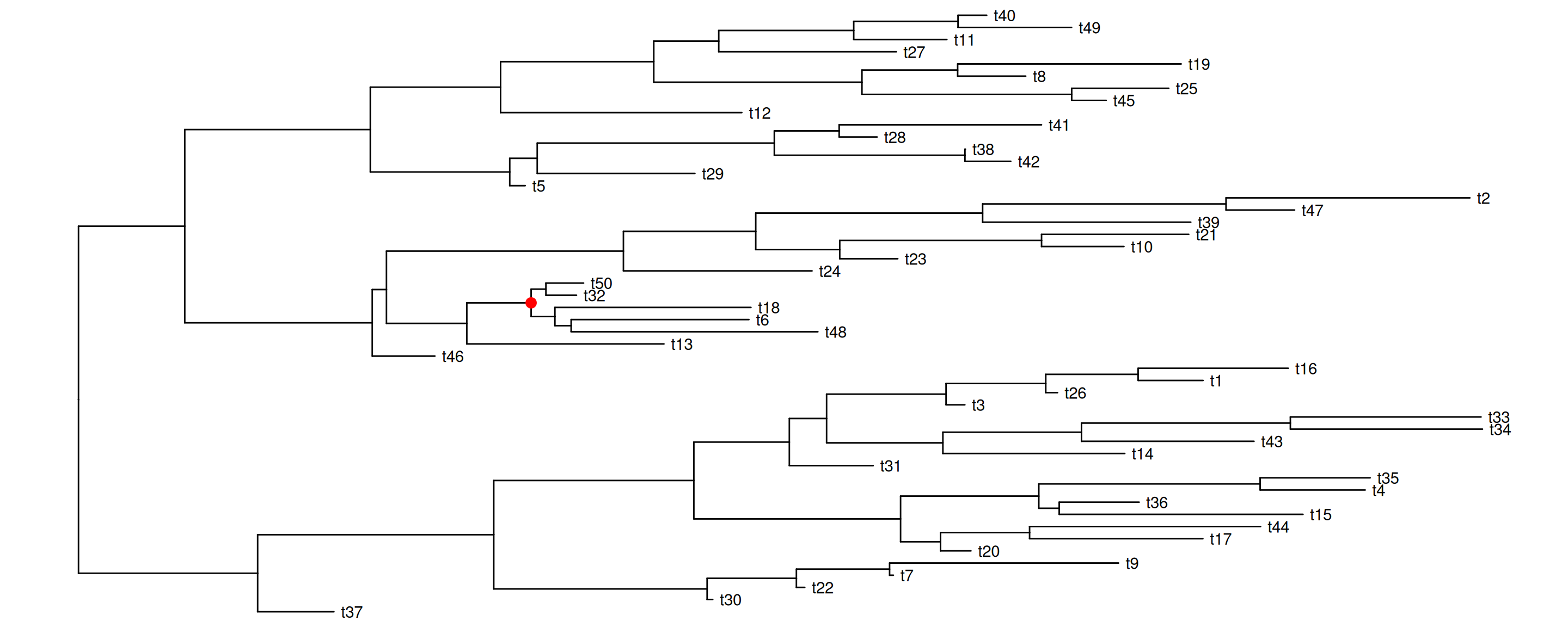
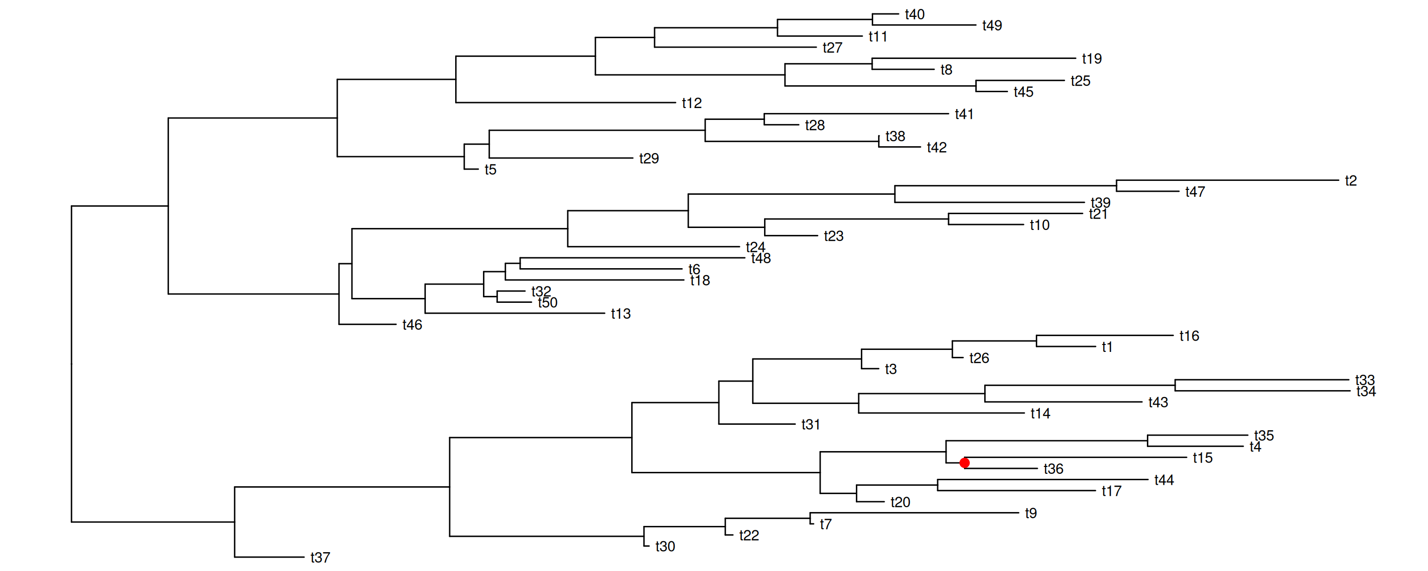
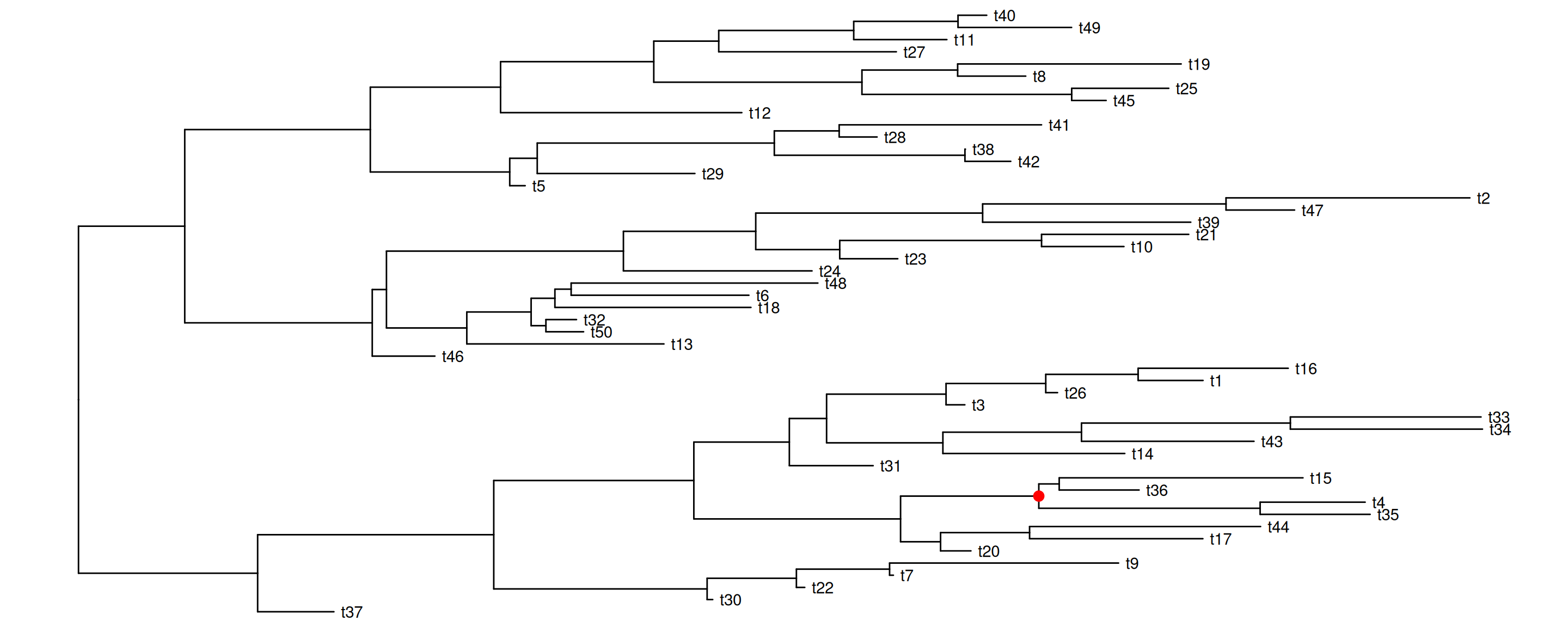
The following example rotates four selected clades (Figure Figure 7.10). It is easy to traverse all the internal nodes and rotate them one-by-one.
set.seed(2016-05-29)x <-rtree(50)p <-ggtree(x) +geom_tiplab()## nn <- unique(reorder(x, 'postorder')$edge[,1]) ## to traverse all the internal nodesnn <-sample(unique(reorder(x, 'postorder')$edge[,1]), 4)pp <-lapply(nn, function(n) { p <-rotate(p, n) p +geom_point2(aes(subset=(node == n)), color='red', size=3)})pp[[1]]pp[[2]]pp[[3]]pp[[4]]
(a) Rotation 1
(b) Rotation 2
(c) Rotation 3
(d) Rotation 4
Figure 7.10: Rotate selected clades. Four clades were randomly selected to rotate (indicated by the red symbol).
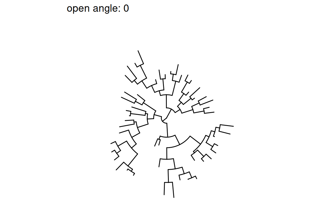
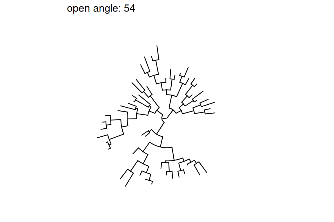
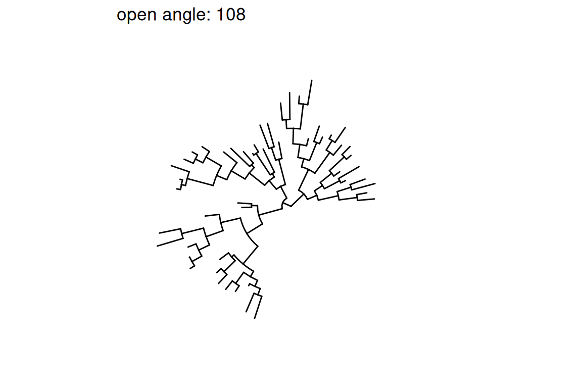
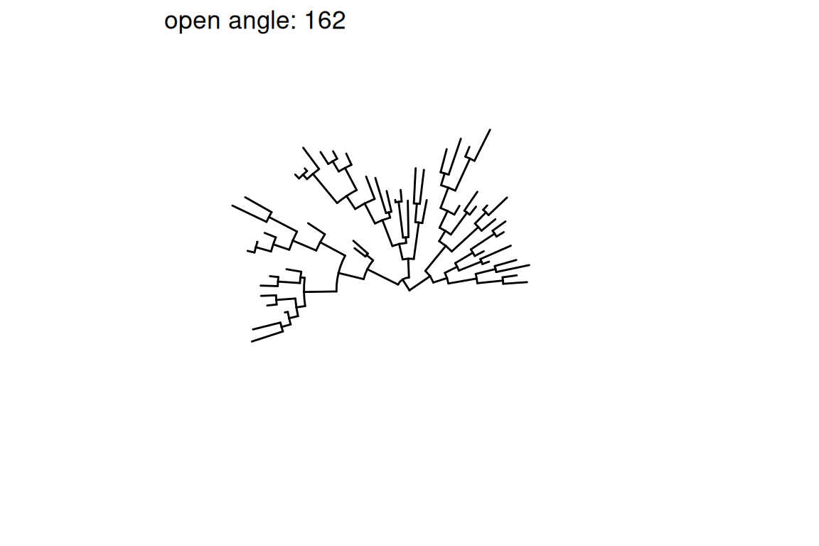
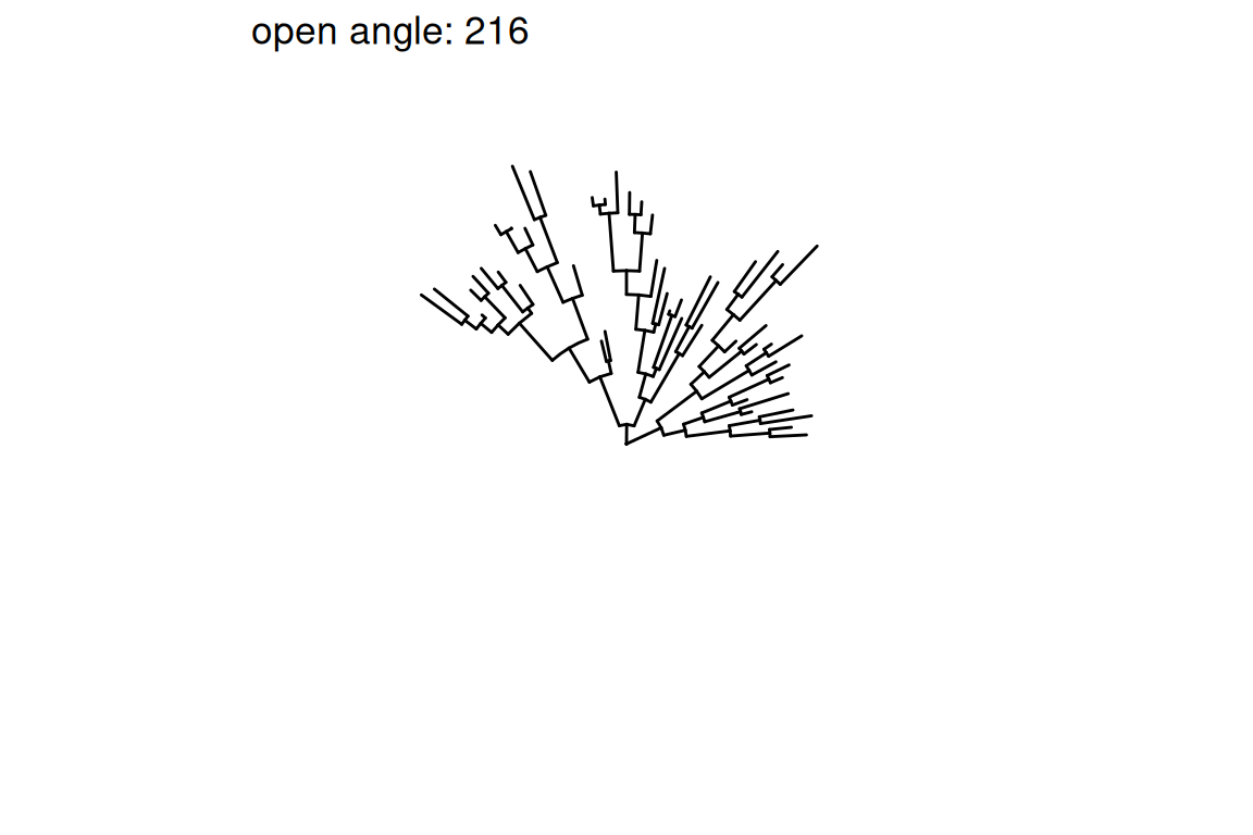
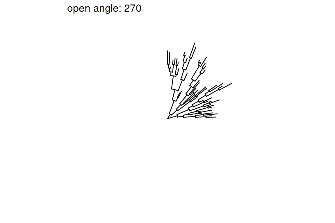
Figure Figure 7.11 demonstrates the usage of open_tree() with different open angles.
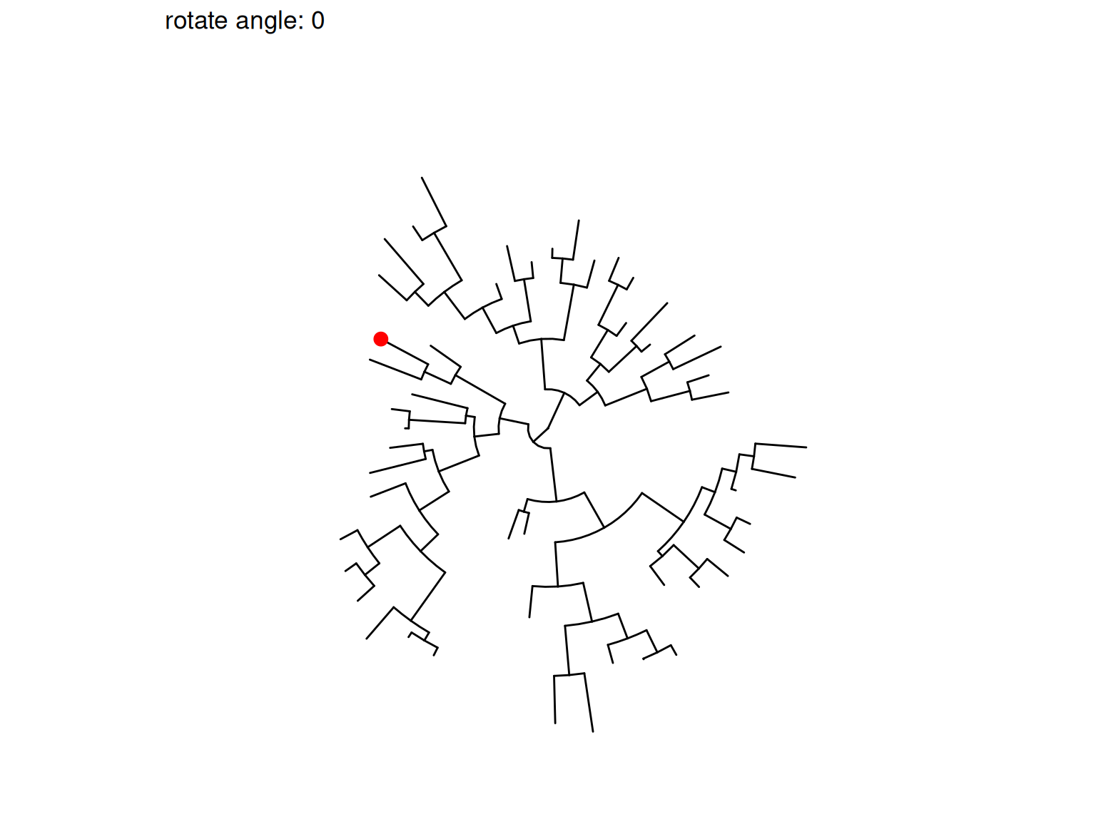
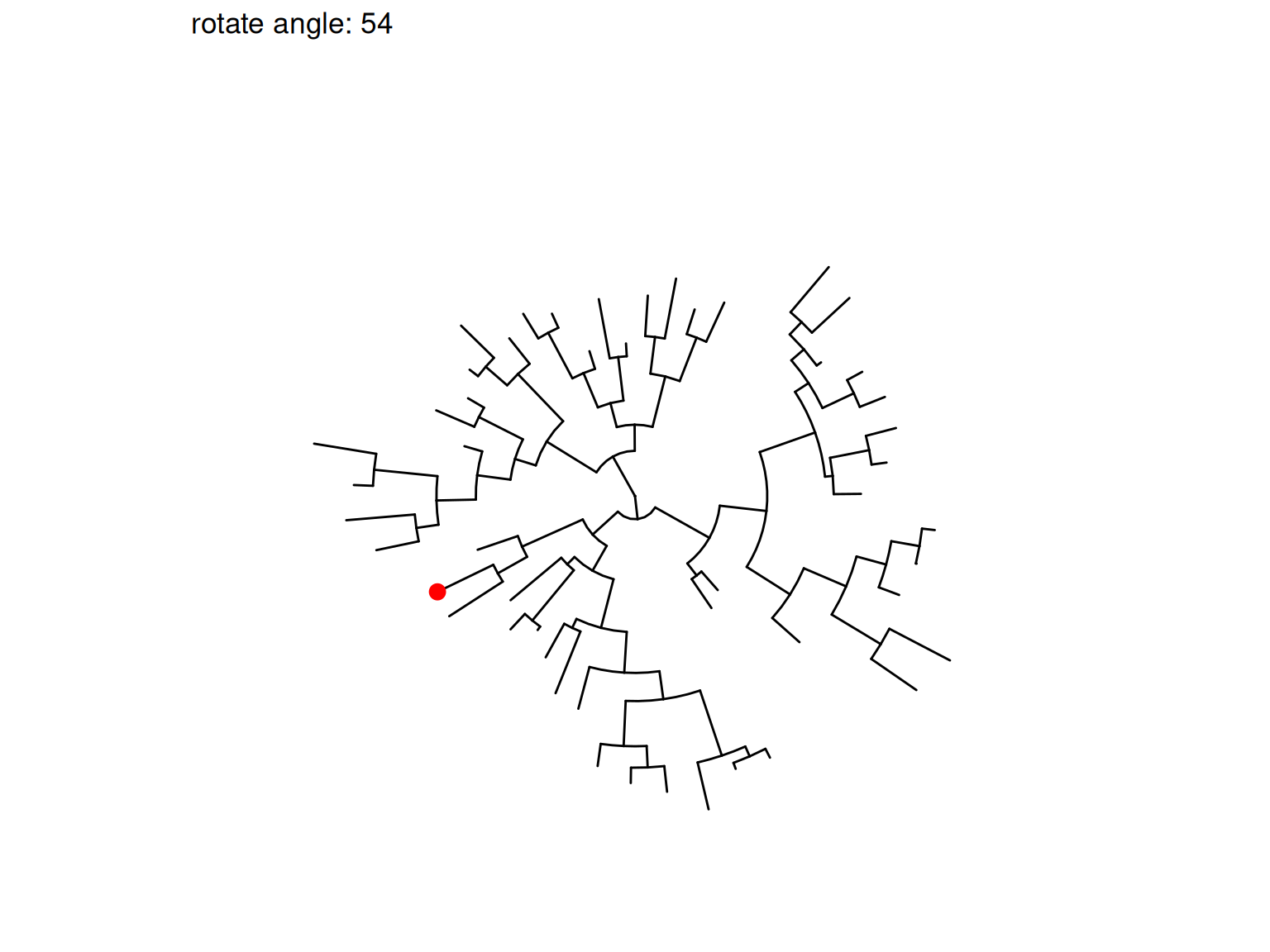
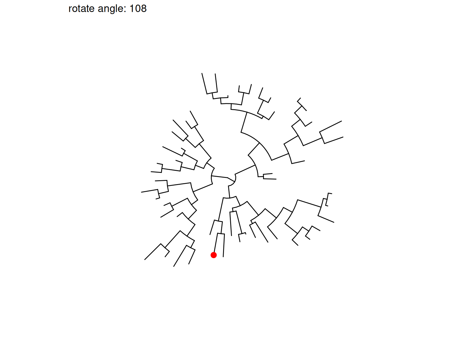
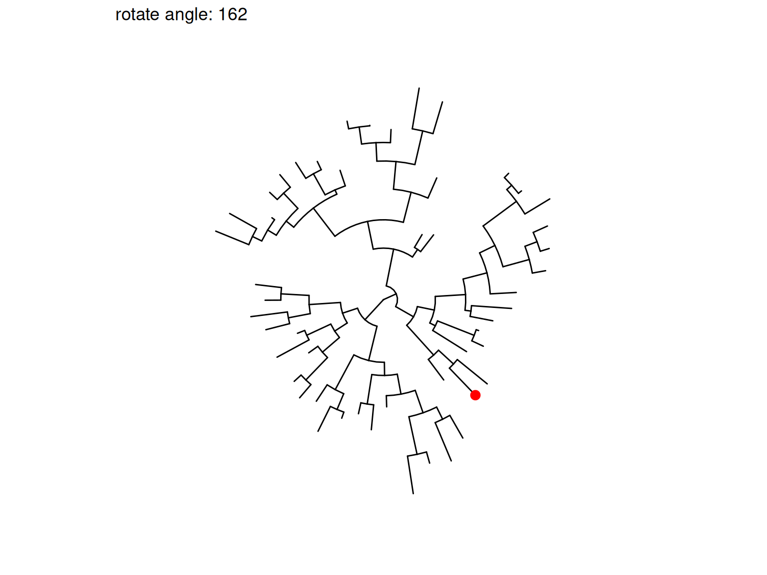
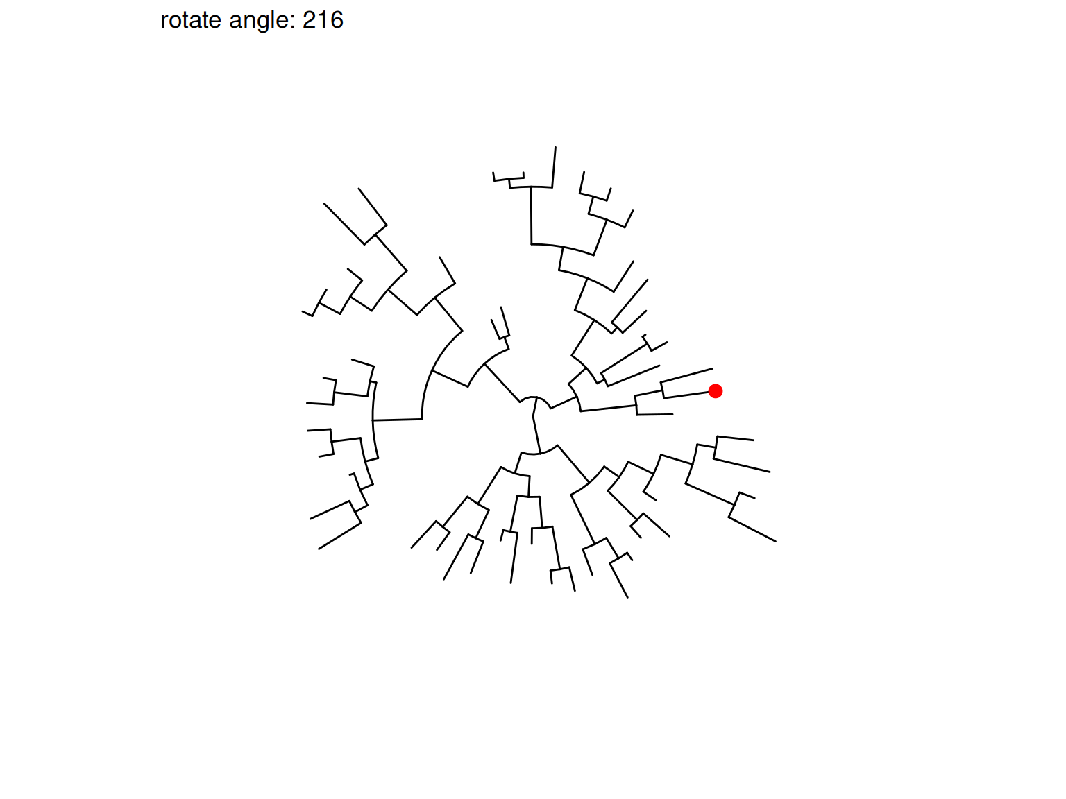
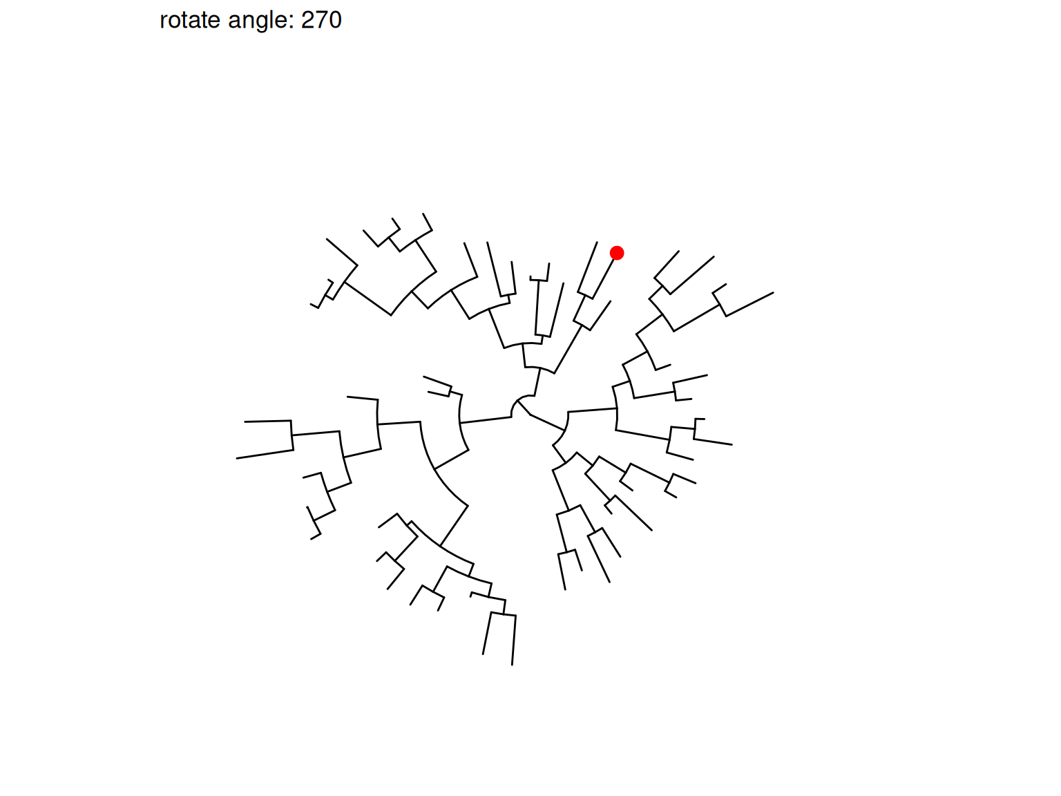
Figure Figure 7.12 illustrates a rotating tree with different angles.
(a)
(b)
(c)
(d)
(e)
(f)
Figure 7.12: Rotate tree with different angles.
Interactive tree manipulation is also possible via the identify() method (see details described in Chapter 12).
7.6 Summary
A good visualization tool can not only help users to present the data, but it should also be able to help users to explore the data. Data exploration can allow users to better understand the data and also help discover hidden patterns. The ggtree provides a set of functions to allow visually manipulating phylogenetic trees and exploring tree structures with associated data. Exploring data in the evolutionary context may help discover new systematic patterns and generate new hypotheses.
Yu, G., Smith, D. K., Zhu, H., Guan, Y., & Lam, T. T.-Y. (2017). Ggtree: An r package for visualization and annotation of phylogenetic trees with their covariates and other associated data. Methods in Ecology and Evolution, 8(1), 28–36. https://doi.org/10.1111/2041-210X.12628