7 Phylogenetic Tree Annotation

library("kableExtra")
library("ape")
library("ggplot2")
library("cowplot")
library("treeio")

treeio v1.35.0 Learn more at https://yulab-smu.top/contribution-tree-data/

Please cite:

LG Wang, TTY Lam, S Xu, Z Dai, L Zhou, T Feng, P Guo, CW Dunn, BR
Jones, T Bradley, H Zhu, Y Guan, Y Jiang, G Yu. treeio: an R package
for phylogenetic tree input and output with richly annotated and
associated data. Molecular Biology and Evolution. 2020, 37(2):599-603.
doi: 10.1093/molbev/msz240

library("ggtree")

ggtree v4.1.1.004 Learn more at https://yulab-smu.top/contribution-tree-data/

Please cite:

S Xu, Z Dai, P Guo, X Fu, S Liu, L Zhou, W Tang, T Feng, M Chen, L
Zhan, T Wu, E Hu, Y Jiang, X Bo, G Yu. ggtreeExtra: Compact
visualization of richly annotated phylogenetic data. Molecular Biology
and Evolution. 2021, 38(9):4039-4042. doi: 10.1093/molbev/msab166


Attaching package: 'ggtree'

The following object is masked from 'package:ape':

    rotate

library("yulab.utils")
source("software-link.R")

7.1 Visualizing and Annotating Tree Using Grammar of Graphics

The ggtree (Yu et al., 2017) is designed for a more general-purpose or a specific type of tree visualization and annotation. It supports the grammar of graphics implemented in ggplot2 and users can freely visualize/annotate a tree by combining several annotation layers.

library(ggtree)
treetext <- "(((ADH2:0.1[&&NHX:S=human], ADH1:0.11[&&NHX:S=human]):
  0.05 [&&NHX:S=primates:D=Y:B=100],ADHY:
  0.1[&&NHX:S=nematode],ADHX:0.12 [&&NHX:S=insect]):
  0.1[&&NHX:S=metazoa:D=N],(ADH4:0.09[&&NHX:S=yeast],
  ADH3:0.13[&&NHX:S=yeast], ADH2:0.12[&&NHX:S=yeast],
  ADH1:0.11[&&NHX:S=yeast]):0.1[&&NHX:S=Fungi])[&&NHX:D=N];"
tree <- read.nhx(textConnection(treetext))
p = ggtree(tree) + geom_tiplab() + 
  geom_label(aes(x=branch, label=S), fill='lightgreen') + 
  geom_label(aes(label=D), fill='steelblue') + 
  geom_text(aes(label=B), hjust=-.5)
p <- p + xlim(NA, 0.28)

library(ggtree)
treetext = "(((ADH2:0.1[&&NHX:S=human], ADH1:0.11[&&NHX:S=human]):
0.05 [&&NHX:S=primates:D=Y:B=100],ADHY:
0.1[&&NHX:S=nematode],ADHX:0.12 [&&NHX:S=insect]):
0.1[&&NHX:S=metazoa:D=N],(ADH4:0.09[&&NHX:S=yeast],
ADH3:0.13[&&NHX:S=yeast], ADH2:0.12[&&NHX:S=yeast],
ADH1:0.11[&&NHX:S=yeast]):0.1[&&NHX:S=Fungi])[&&NHX:D=N];"
tree <- read.nhx(textConnection(treetext))
ggtree(tree) + geom_tiplab() + 
  geom_label(aes(x=branch, label=S), fill='lightgreen') + 
  geom_label(aes(label=D), fill='steelblue') + 
  geom_text(aes(label=B), hjust=-.5)

Figure 7.1: **Annotating tree using the grammar of graphics.** The NHX tree was annotated using the grammar of graphic syntax by combining different layers using the `+` operator. Species information was labeled in the middle of the branches. Duplication events were shown on the most recent common ancestor and clade bootstrap values were displayed near to it.

Here, as an example, we visualized the tree with several layers to display annotation stored in NHX tags, including a layer of geom_tiplab() to display tip labels (gene name in this case), a layer using geom_label() to show species information (S tag) colored by light green, a layer of duplication event information (D tag) colored by steelblue and another layer using geom_text() to show bootstrap value (B tag).

Layers defined in ggplot2 can be applied to ggtree directly as demonstrated in Figure Figure 7.1 of using geom_label() and geom_text(). But ggplot2 does not provide graphic layers that are specifically designed for phylogenetic tree annotation. For instance, layers for tip labels, tree branch scale legend, highlight, or labeling clade are all unavailable. To make tree annotation more flexible, several layers have been implemented in ggtree (Table Table 5.1), enabling different ways of annotation on various parts/components of a phylogenetic tree.

Geom layers defined in ggtree.
Layer	Description
geom_balance	Highlights the two direct descendant clades of an internal node
geom_cladelab	Annotates a clade with bar and text label (or image)
geom_facet	Plots associated data in a specific panel (facet) and aligns the plot with the tree
geom_hilight	Highlights selected clade with rectangular or round shape
geom_inset	Adds insets (subplots) to tree nodes
geom_label2	The modified version of geom_label, with subset aesthetic supported
geom_nodepoint	Annotates internal nodes with symbolic points
geom_point2	The modified version of geom_point, with subset aesthetic supported
geom_range	Bar layer to present uncertainty of evolutionary inference
geom_rootpoint	Annotates root node with symbolic point
geom_rootedge	Adds root-edge to a tree
geom_segment2	The modified version of geom_segment, with subset aesthetic supported
geom_strip	Annotates associated taxa with bar and (optional) text label
geom_taxalink	Links related taxa
geom_text2	The modified version of geom_text, with subset aesthetic supported
geom_tiplab	The layer of tip labels
geom_tippoint	Annotates external nodes with symbolic points
geom_tree	Tree structure layer, with multiple layouts supported
geom_treescale	Tree branch scale legend

7.2 Layers for Tree Annotation

7.2.1 Colored strips

The ggtree (Yu et al., 2017) implements geom_cladelab() layer to annotate a selected clade with a bar indicating the clade with a corresponding label.

The geom_cladelab() layer accepts a selected internal node number and labels the corresponding clade automatically (Figure Figure 7.2 (a)). To get the internal node number, please refer to Chapter 2.

set.seed(2015-12-21)
tree <- rtree(30)
p <- ggtree(tree) + xlim(NA, 8)

p + geom_cladelab(node=45, label="test label") +
    geom_cladelab(node=34, label="another clade")

Users can set the parameter, align = TRUE, to align the clade label, offset, to adjust the position and color to set the color of the bar and label text, etc. (Figure Figure 7.2 (b)).

p + geom_cladelab(node=45, label="test label", align=TRUE,  
                  offset = .2, textcolor='red', barcolor='red') +
    geom_cladelab(node=34, label="another clade", align=TRUE, 
                  offset = .2, textcolor='blue', barcolor='blue')

Users can change the angle of the clade label text and relative position from text to bar via the parameter offset.text. The size of the bar and text can be changed via the parameters barsize and fontsize, respectively (Figure Figure 7.2 (c)).

p + geom_cladelab(node=45, label="test label", align=TRUE, angle=270, 
            hjust='center', offset.text=.5, barsize=1.5, fontsize=8) +
    geom_cladelab(node=34, label="another clade", align=TRUE, angle=45)

Warning: Using `size` aesthetic for lines was deprecated in ggplot2 3.4.0.
ℹ Please use `linewidth` instead.
ℹ The deprecated feature was likely used in the ggtree package.
  Please report the issue at <https://github.com/YuLab-SMU/ggtree/issues>.

Users can also use geom_label() to label the text and can set the background color by fill parameter (Figure Figure 7.2 (d)).

p + geom_cladelab(node=34, label="another clade", align=TRUE, 
                  geom='label', fill='lightblue')

Warning in (function (mapping = NULL, data = NULL, ..., stat = "identity", :
Ignoring unknown parameters: `label.size`

Warning in (function (mapping = NULL, data = NULL, ..., stat = "identity", :
Ignoring unknown parameters: `label.size`

In addition, geom_cladelab() allows users to use the image or phylopic to annotate the clades, and supports using aesthetic mapping to automatically annotate the clade with bar and text label or image (e.g., mapping variable to color the clade labels) (Figure Figure 7.3).

dat <- data.frame(node = c(45, 34), 
            name = c("test label", "another clade"))
# The node and label is required when geom="text" 
## or geom="label" or geom="shadowtext".
p1 <- p + geom_cladelab(data = dat, 
        mapping = aes(node = node, label = name, color = name), 
        fontsize = 3)

dt <- data.frame(node = c(45, 34), 
                 image = c("7fb9bea8-e758-4986-afb2-95a2c3bf983d", 
                          "0174801d-15a6-4668-bfe0-4c421fbe51e8"), 
                 name = c("specie A", "specie B"))

# when geom="phylopic" or geom="image", the image of aes is required.
p2 <- p + geom_cladelab(data = dt, 
                mapping = aes(node = node, label = name, image = image), 
                geom = "phylopic", imagecolor = "black", 
                offset=1, offset.text=0.5)

# The color or size of image also can be mapped.
p3 <- p + geom_cladelab(data = dt, 
              mapping = aes(node = node, label = name, 
                          image = image, color = name), 
              geom = "phylopic", offset = 1, offset.text=0.5)

(a) Use aesthetic mapping to annotate clades

The geom_cladelab() layer also supports unrooted tree layouts (Figure Figure 7.4 (a)).

ggtree(tree, layout="daylight") + 
  geom_cladelab(node=35, label="test label", angle=0, 
                  fontsize=8, offset=.5, vjust=.5)  + 
  geom_cladelab(node=55, label='another clade', 
                  angle=-95, hjust=.5, fontsize=8)

The geom_cladelab() is designed for labeling Monophyletic (Clade) while there are related taxa that do not form a clade. In ggtree, we provide another layer, geom_strip(), to add a strip/bar to indicate the association with an optional label for Polyphyletic or Paraphyletic (Figure Figure 7.4 (b)).

p + geom_tiplab() + 
  geom_strip('t10', 't30', barsize=2, color='red', 
            label="associated taxa", offset.text=.1) + 
  geom_strip('t1', 't18', barsize=2, color='blue', 
            label = "another label", offset.text=.1)

(a) geom_cladelab() supports unrooted layouts

7.2.2 Highlight clades

The ggtree implements the geom_hilight() layer, which accepts an internal node number and adds a layer of a rectangle to highlight the selected clade (Figure Figure 7.5)¹.

nwk <- system.file("extdata", "sample.nwk", package="treeio")
tree <- read.tree(nwk)
ggtree(tree) + 
    geom_hilight(node=21, fill="steelblue", alpha=.6) +
    geom_hilight(node=17, fill="darkgreen", alpha=.6)

ggtree(tree, layout="circular") + 
    geom_hilight(node=21, fill="steelblue", alpha=.6) +
    geom_hilight(node=23, fill="darkgreen", alpha=.6)

The geom_hilight layer also supports highlighting clades for unrooted layout trees with round (‘encircle’) or rectangular (‘rect’) shape (Figure Figure 7.5 (c)).

## type can be 'encircle' or 'rect'
pg + geom_hilight(node=55, linetype = 3) + 
  geom_hilight(node=35, fill='darkgreen', type="rect")

Another way to highlight selected clades is by setting the clades with different colors and/or line types as demonstrated in Figure Figure 8.2.

In addition to geom_hilight(), ggtree also implements geom_balance() which is designed to highlight neighboring subclades of a given internal node (Figure Figure 7.5 (d)).

ggtree(tree) +
  geom_balance(node=16, fill='steelblue', color='white', alpha=0.6, extend=1) +
  geom_balance(node=19, fill='darkgreen', color='white', alpha=0.6, extend=1)

The geom_hilight() layer supports using aesthetic mapping to automatically highlight clades as demonstrated in Figures Figure 7.5 (e) and Figure 7.5 (f). For plot in Cartesian coordinates (e.g., rectangular layout), the rectangle can be rounded (Figure Figure 7.5 (e)) or filled with gradient colors (Figure Figure 7.5 (f)).

## using external data
d <- data.frame(node=c(17, 21), type=c("A", "B"))
ggtree(tree) + geom_hilight(data=d, aes(node=node, fill=type),
                            type = "roundrect")

## using data stored in the tree object
x <- read.nhx(system.file("extdata/NHX/ADH.nhx", package="treeio"))
ggtree(x) + geom_hilight(mapping=aes(subset = node %in% c(10, 12), 
                                    fill = S),
                        type = "gradient", gradient.direction = 'rt',
                        alpha = .8) +
  scale_fill_manual(values=c("steelblue", "darkgreen"))

7.2.3 Taxa connection

Some evolutionary events (e.g., reassortment, horizontal gene transfer) cannot be modeled by a simple tree. The ggtree provides the geom_taxalink() layer that allows drawing straight or curved lines between any of two nodes in the tree, allowing it to represent evolutionary events by connecting taxa. It works with rectangular (Figure Figure 7.6 (a)), circular (Figure Figure 7.6 (b)), and inward circular (Figure Figure 7.6 (c)) layouts. The geom_taxalink() is not only useful for presenting evolutionary events, but it can also be used to combine evolutionary trees to present relationships or interactions between species (Xu et al., 2021).

The geom_taxalink() layout supports aesthetic mapping, which requires a data.frame that stores association information with/without meta-data as input (Figure Figure 7.6 (d)).

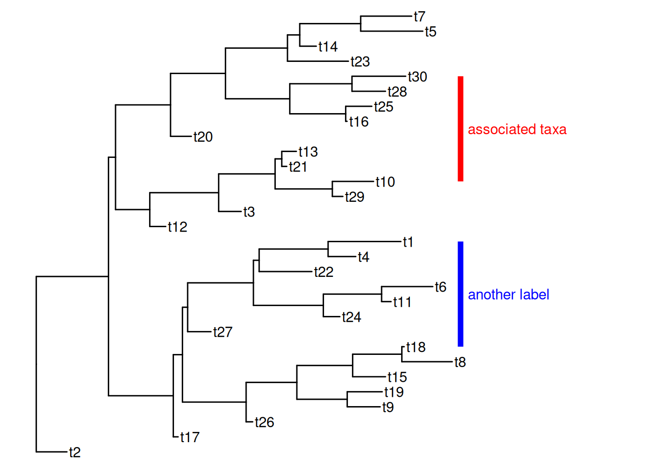
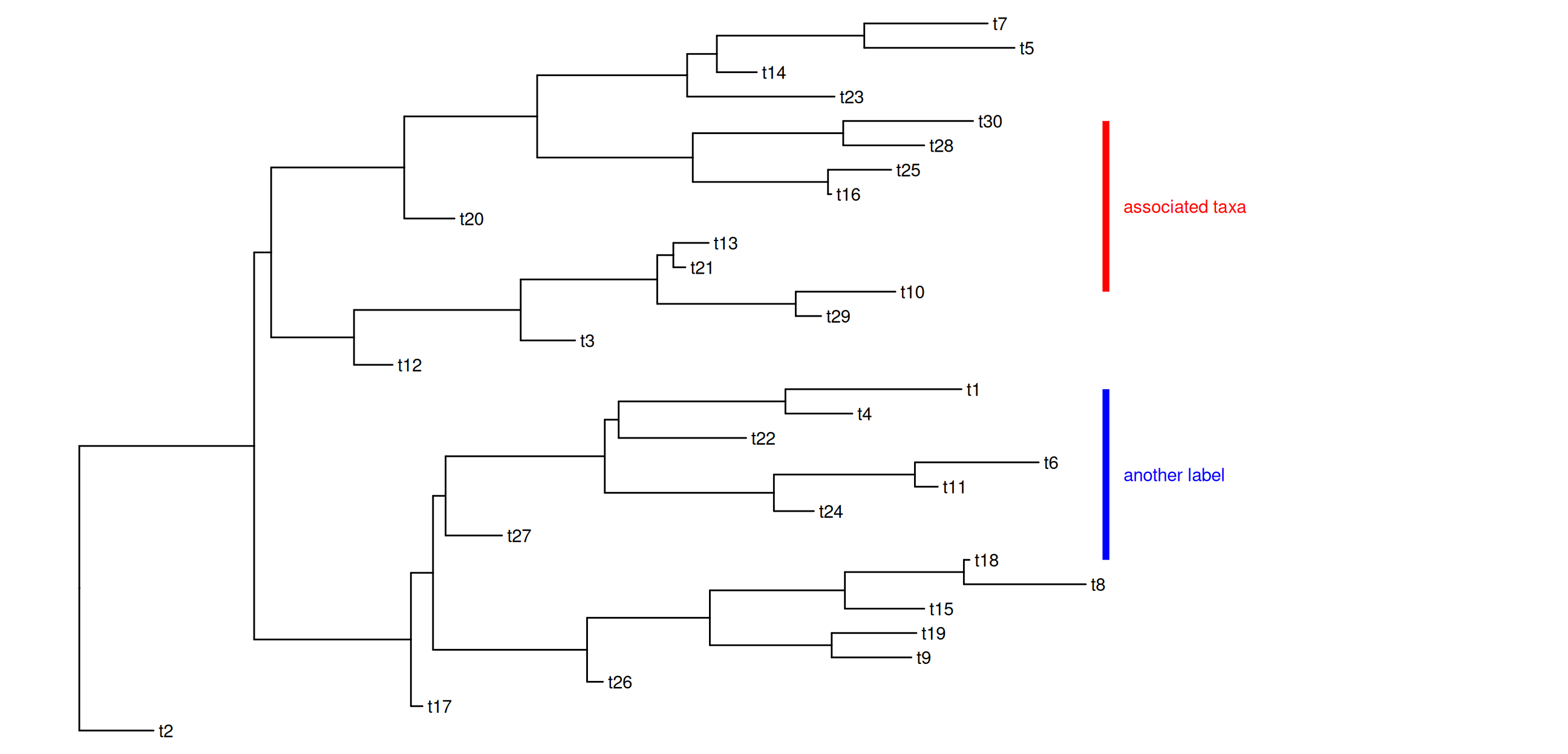
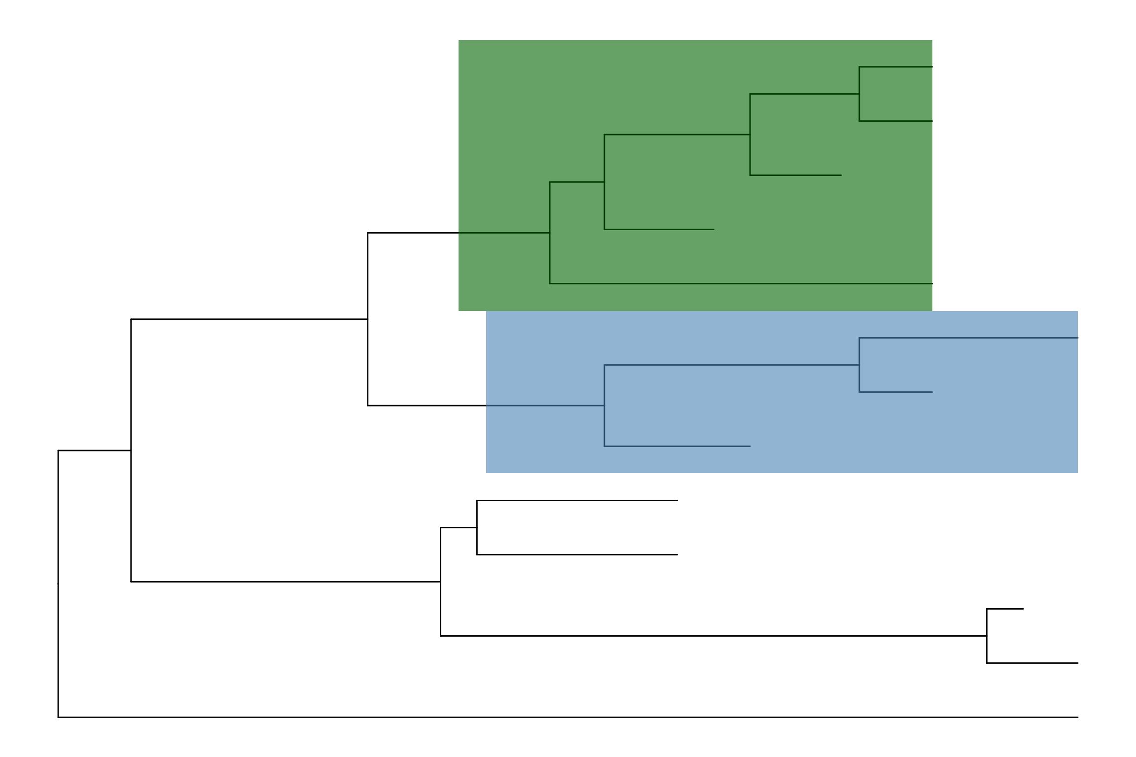
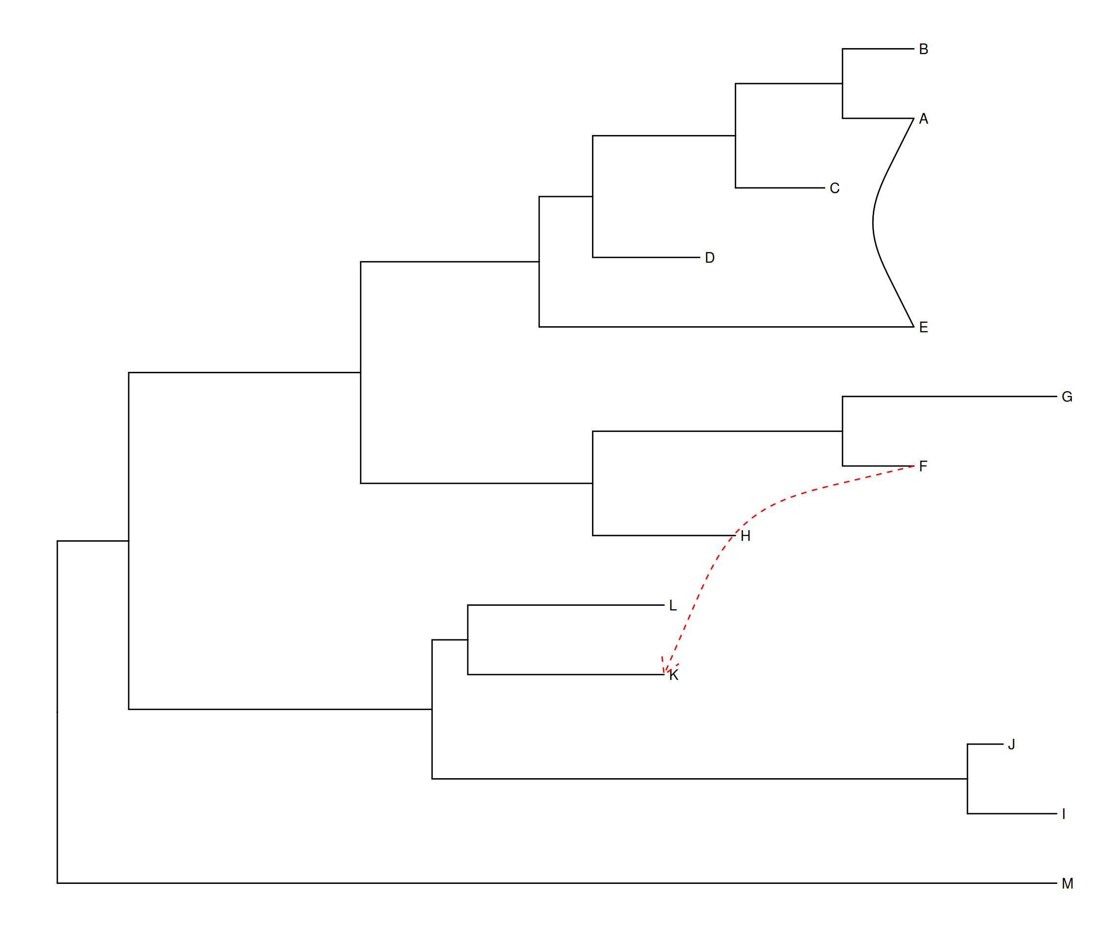
p1 <- ggtree(tree) + geom_tiplab() + geom_taxalink(taxa1='A', taxa2='E') + 
  geom_taxalink(taxa1='F', taxa2='K', color='red', linetype = 'dashed',
    arrow=arrow(length=unit(0.02, "npc")))

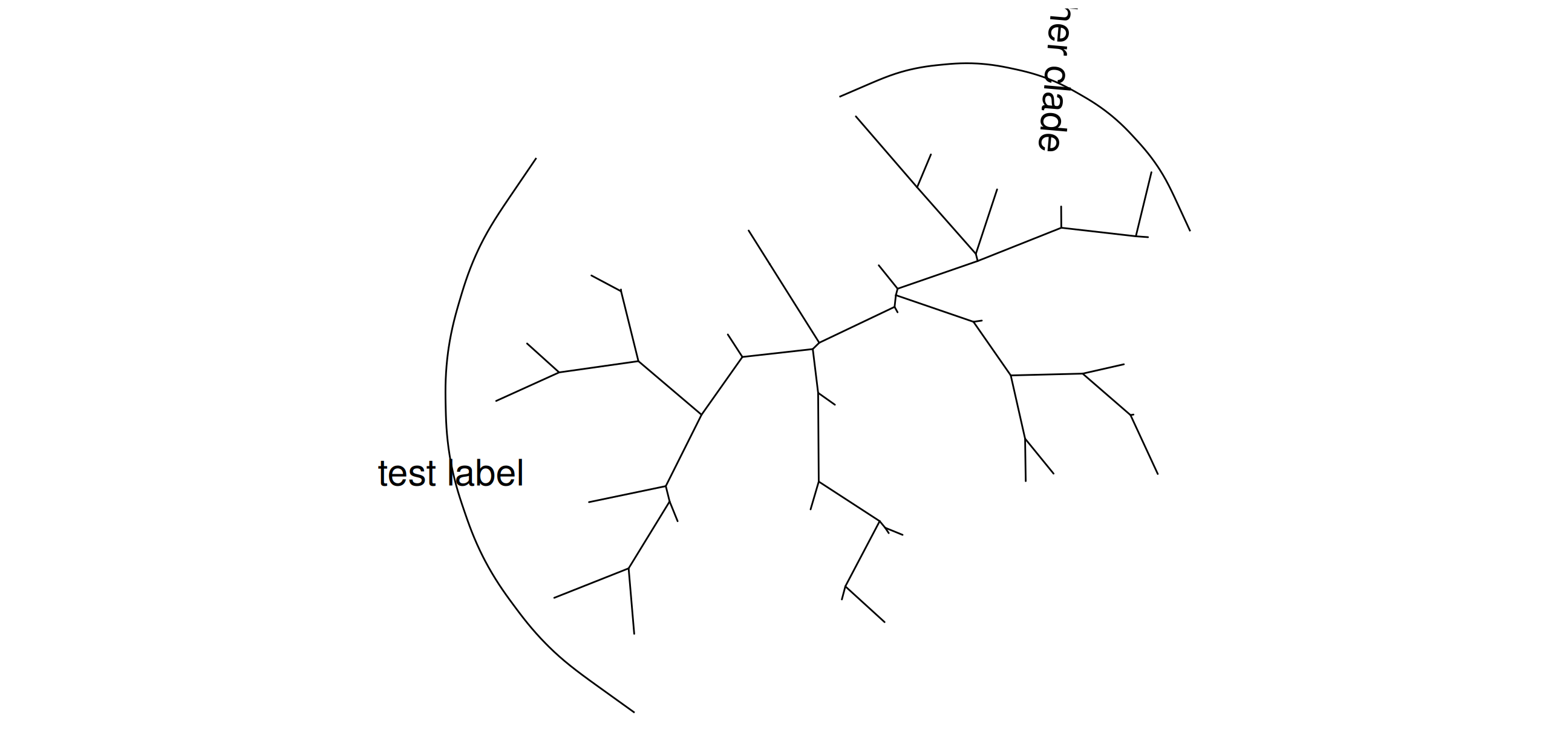
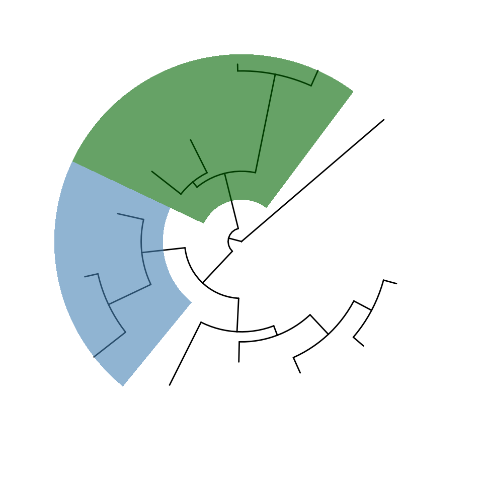
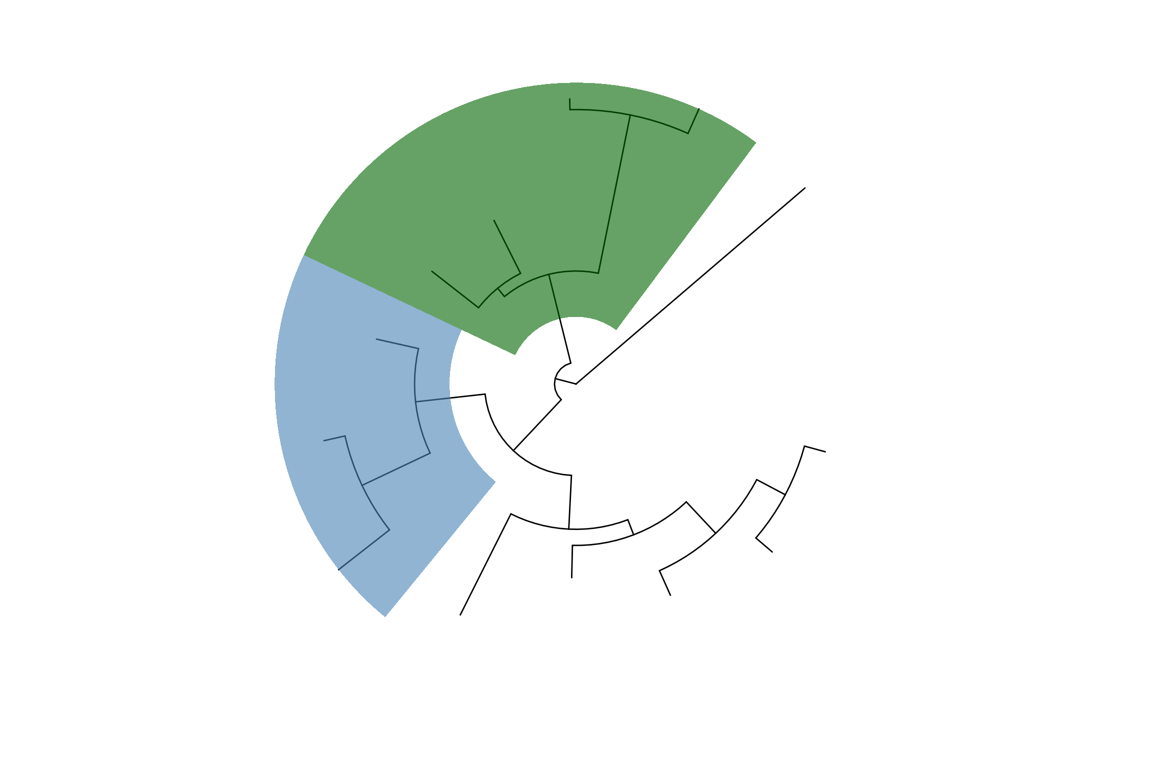
p2 <- ggtree(tree, layout="circular") + 
      geom_taxalink(taxa1='A', taxa2='E', color="grey", alpha=0.5, 
                offset=0.05, arrow=arrow(length=unit(0.01, "npc"))) + 
      geom_taxalink(taxa1='F', taxa2='K', color='red', 
                linetype = 'dashed', alpha=0.5, offset=0.05,
                arrow=arrow(length=unit(0.01, "npc"))) +
      geom_taxalink(taxa1="L", taxa2="M", color="blue", alpha=0.5, 
                offset=0.05, hratio=0.8, 
                arrow=arrow(length=unit(0.01, "npc"))) + 
      geom_tiplab()

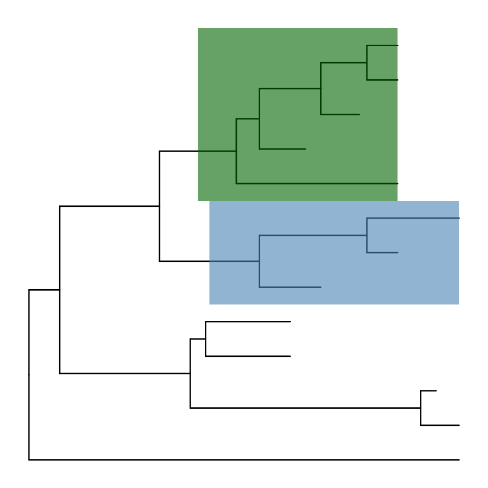
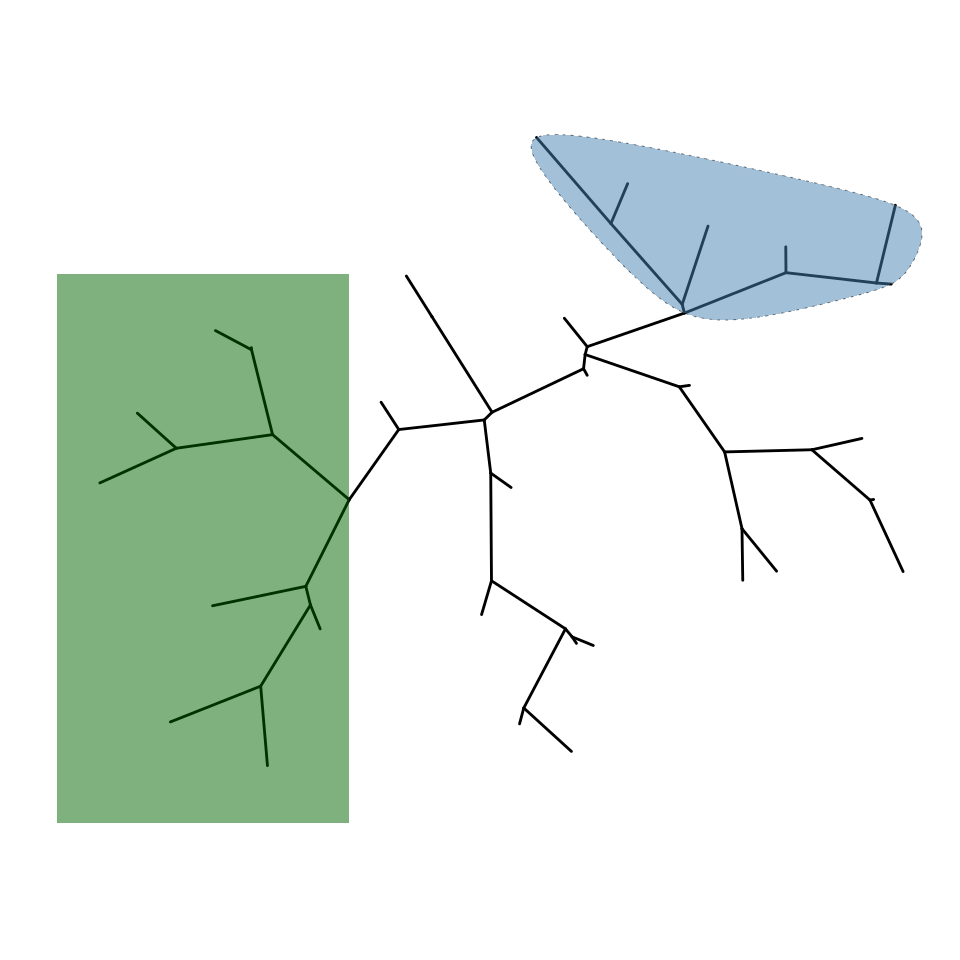
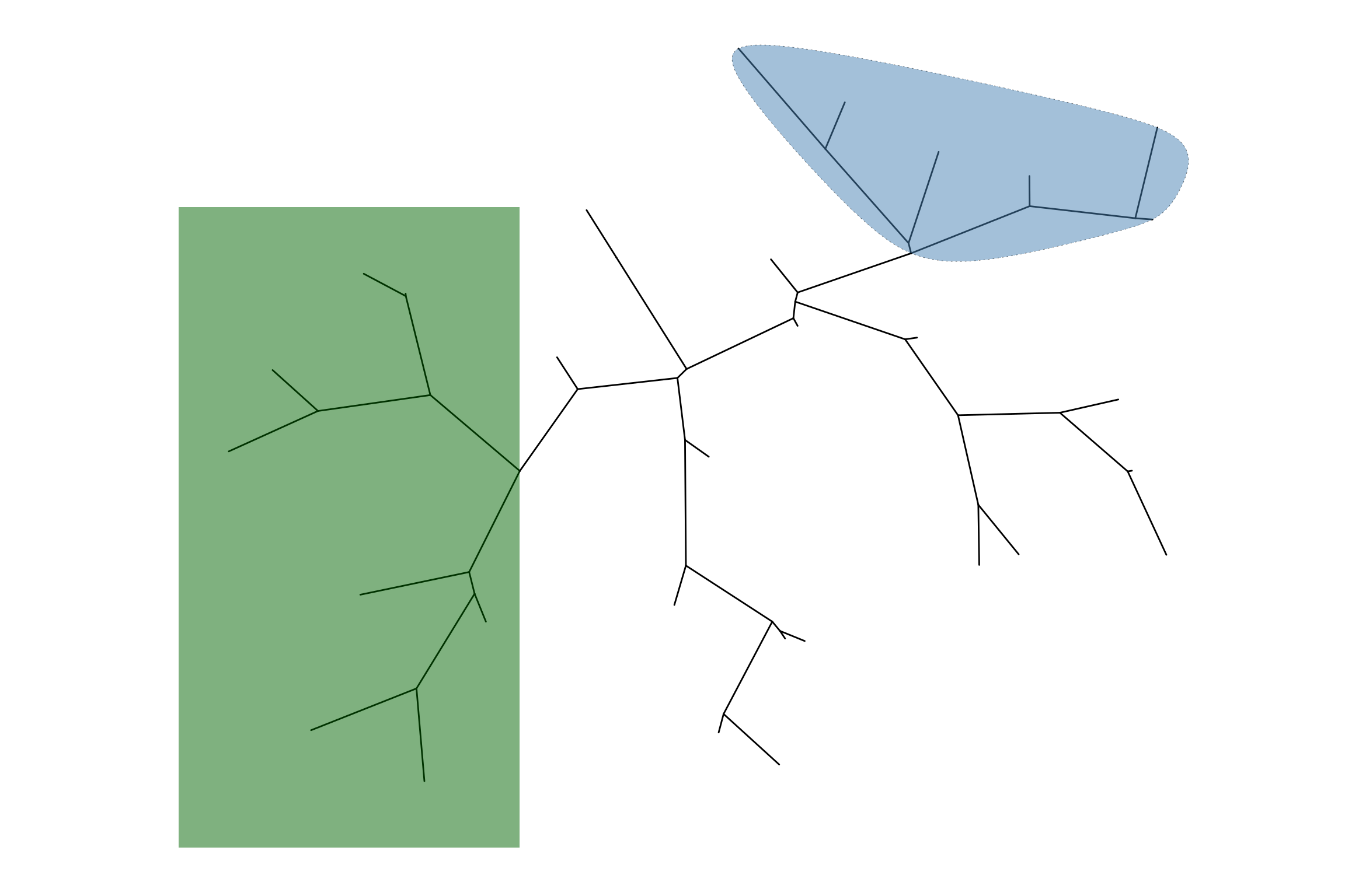
# when the tree was created using reverse x, 
# we can set outward to FALSE, which will generate the inward curve lines.
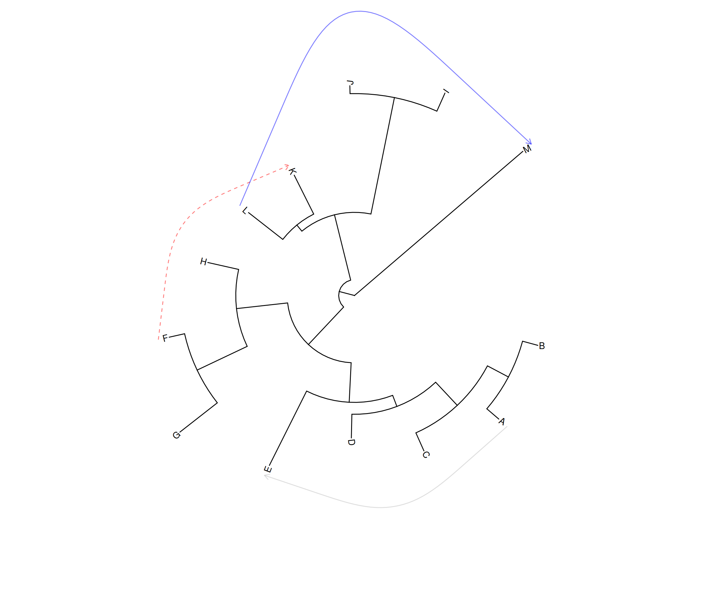
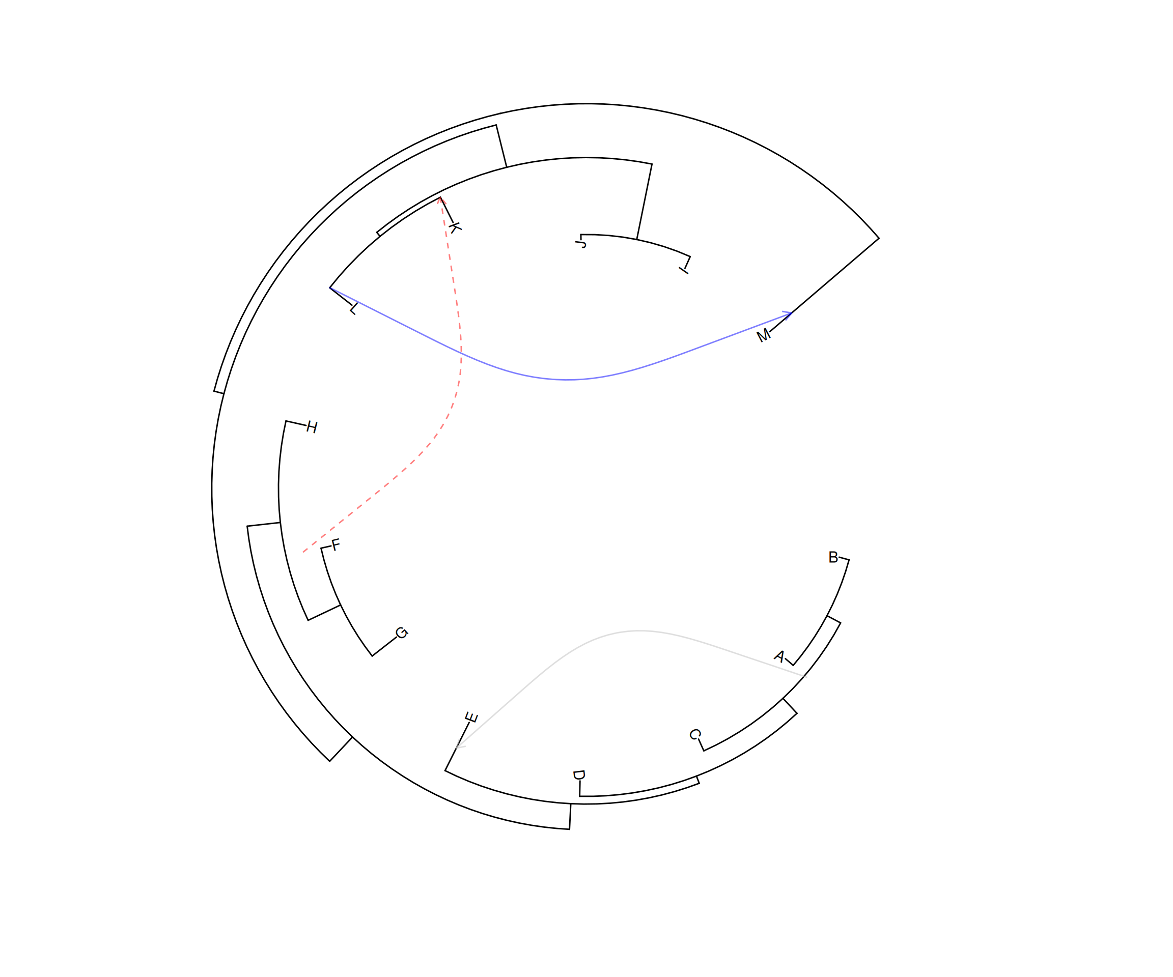
p3 <- ggtree(tree, layout="inward_circular", xlim=150) +
      geom_taxalink(taxa1='A', taxa2='E', color="grey", alpha=0.5, 
                    offset=-0.2, outward=FALSE,
                    arrow=arrow(length=unit(0.01, "npc"))) +
      geom_taxalink(taxa1='F', taxa2='K', color='red', linetype = 'dashed', 
                    alpha=0.5, offset=-0.2, outward=FALSE,
                    arrow=arrow(length=unit(0.01, "npc"))) +
      geom_taxalink(taxa1="L", taxa2="M", color="blue", alpha=0.5, 
                    offset=-0.2, outward=FALSE,
                    arrow=arrow(length=unit(0.01, "npc"))) +
      geom_tiplab(hjust=1) 

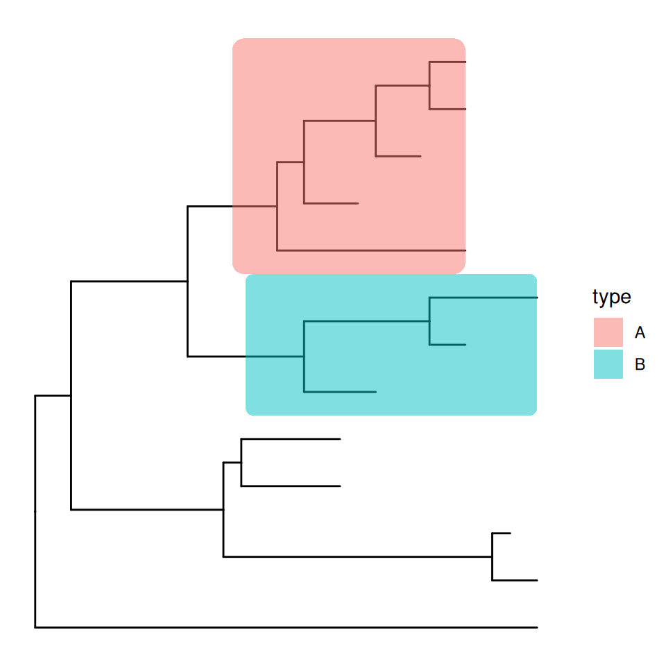
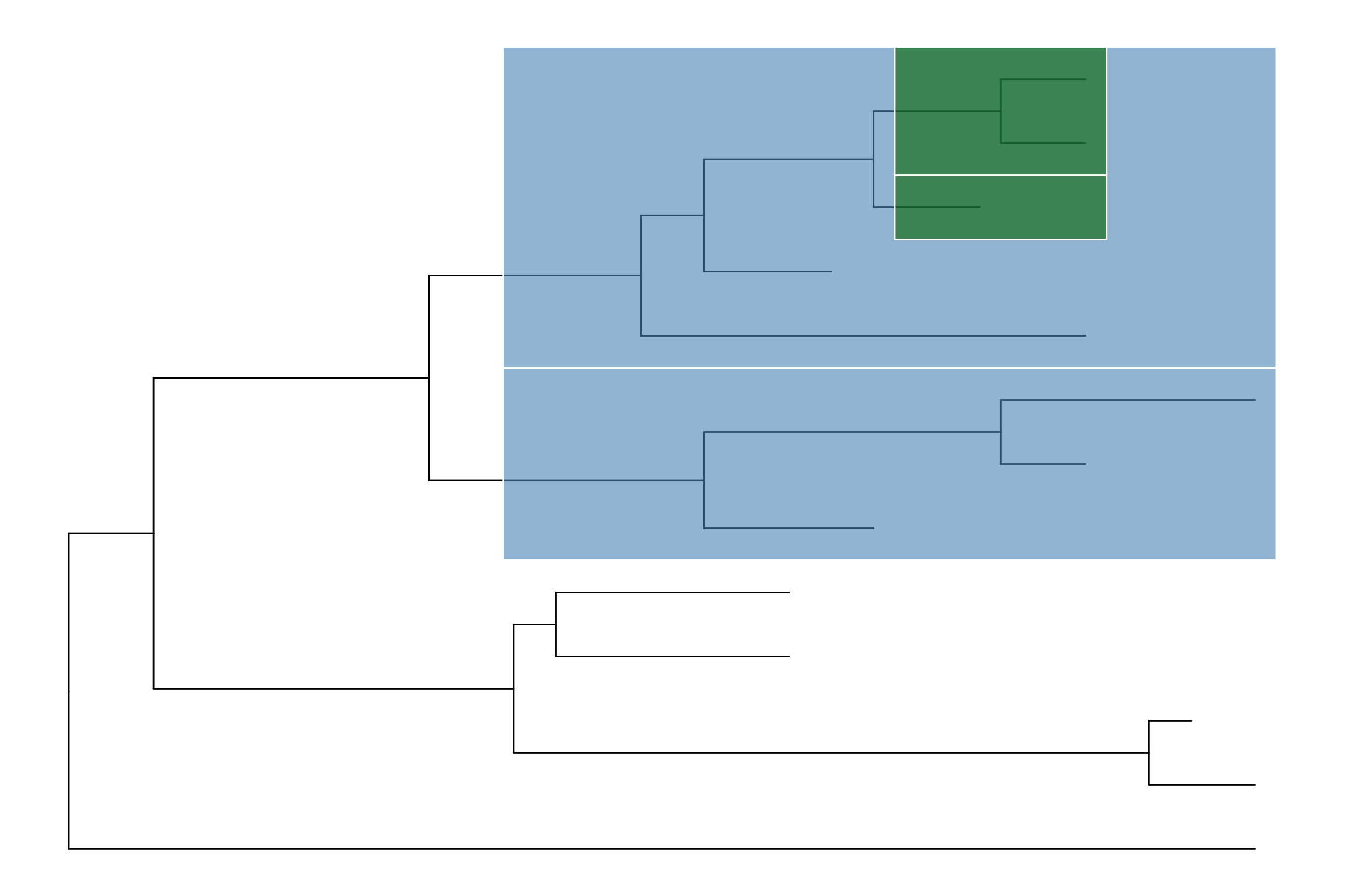
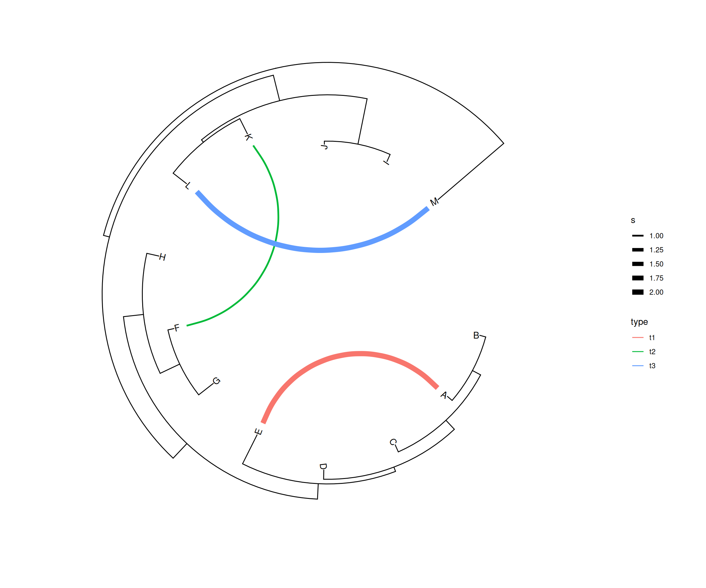
dat <- data.frame(from=c("A", "F", "L"), 
                  to=c("E", "K", "M"), 
                  h=c(1, 1, 0.1), 
                  type=c("t1", "t2", "t3"), 
                  s=c(2, 1, 2))
p4 <- ggtree(tree, layout="inward_circular", xlim=c(150, 0)) +
          geom_taxalink(data=dat, 
                         mapping=aes(taxa1=from, 
                                     taxa2=to, 
                                     color=type, 
                                     size=s), 
                         ncp=10,
                         offset=0.15) + 
          geom_tiplab(hjust=1) +
          scale_size_continuous(range=c(1,3))

p1
p2
p3
p4

7.2.4 Uncertainty of evolutionary inference

The geom_range() layer supports displaying interval (highest posterior density, confidence interval, range) as horizontal bars on tree nodes. The center of the interval will anchor to the corresponding node. The center by default is the mean value of the interval (Figure Figure 7.7 (a)). We can set the center to the estimated mean or median value (Figure Figure 7.7 (b)), or the observed value. As the tree branch and the interval may not be on the same scale, ggtree provides scale_x_range to add a second x-axis for the range (Figure Figure 7.7 (c)). Note that x-axis is disabled by the default theme, and we need to enable it if we want to display it (e.g., using theme_tree2()).

file <- system.file("extdata/MEGA7", "mtCDNA_timetree.nex", package = "treeio")
x <- read.mega(file)
p1 <- ggtree(x) + geom_range('reltime_0.95_CI', color='red', size=3, alpha=.3)
p2 <- ggtree(x) + geom_range('reltime_0.95_CI', color='red', size=3, 
                              alpha=.3, center='reltime')  
p3 <- p2 + scale_x_range() + theme_tree2()

7.3 Tree Annotation with Output from Evolution Software

7.3.1 Tree annotation using data from evolutionary analysis software

Chapter 1 introduced using treeio package (Wang et al., 2020) to parse different tree formats and commonly used software outputs to obtain phylogeny-associated data. These imported data, as S4 objects, can be visualized directly using ggtree. Figure Figure 7.1 demonstrates a tree annotated using the information (species classification, duplication event, and bootstrap value) stored in the NHX file. PHYLDOG and pkg_revbayes output NHX files that can be parsed by treeio and visualized by ggtree with annotation using their inference data.

Furthermore, the evolutionary data from the inference of BEAST, MrBayes, and RevBayes, d_N/d_S values inferred by CODEML, ancestral sequences inferred by HyPhy, CODEML, or BASEML and short read placement by EPA and PPLACER can be used to annotate the tree directly.

file <- system.file("extdata/BEAST", "beast_mcc.tree", package="treeio")
beast <- read.beast(file)
ggtree(beast, aes(color=rate))  +
    geom_range(range='length_0.95_HPD', color='red', alpha=.6, size=2) +
    geom_nodelab(aes(x=branch, label=round(posterior, 2)), vjust=-.5, size=3) +
    scale_color_continuous(low="darkgreen", high="red") +
    theme(legend.position=c(.1, .8))

Figure 7.8: **Annotating `r pkg_beast` tree with *length_95%_HPD* and posterior.** Branch length credible intervals (95% HPD) were displayed as red horizontal bars and clade posterior values were shown on the middle of branches.

In Figure Figure 7.8, the tree was visualized and annotated with posterior >0.9 and demonstrated length uncertainty (95% Highest Posterior Density (HPD) interval).

Ancestral sequences inferred by HyPhy can be parsed using treeio, whereas the substitutions along each tree branch were automatically computed and stored inside the phylogenetic tree object (i.e., S4 object). The ggtree package can utilize this information stored in the object to annotate the tree, as demonstrated in Figure Figure 7.9.

nwk <- system.file("extdata/HYPHY", "labelledtree.tree", 
                   package="treeio")
ancseq <- system.file("extdata/HYPHY", "ancseq.nex", 
                      package="treeio")
tipfas <- system.file("extdata", "pa.fas", package="treeio")
hy <- read.hyphy(nwk, ancseq, tipfas)
ggtree(hy) + 
  geom_text(aes(x=branch, label=AA_subs), size=2, 
            vjust=-.3, color="firebrick")

Figure 7.9: **Annotating tree with amino acid substitution determined by ancestral sequences inferred by `r pkg_hyphy`.** Amino acid substitutions were displayed in the middle of branches.

PAML’s BASEML and CODEML can also be used to infer ancestral sequences, whereas CODEML can infer selection pressure. After parsing this information using treeio, ggtree can integrate this information into the same tree structure and be used for annotation as illustrated in Figure Figure 7.10.

rstfile <- system.file("extdata/PAML_Codeml", "rst", 
                       package="treeio")
mlcfile <- system.file("extdata/PAML_Codeml", "mlc", 
                       package="treeio")
ml <- read.codeml(rstfile, mlcfile)
ggtree(ml, aes(color=dN_vs_dS), branch.length='dN_vs_dS') + 
  scale_color_continuous(name='dN/dS', limits=c(0, 1.5),
                         oob=scales::squish,
                         low='darkgreen', high='red') +
  geom_text(aes(x=branch, label=AA_subs), 
            vjust=-.5, color='steelblue', size=2) +
  theme_tree2(legend.position=c(.9, .3))

Figure 7.10: **Annotating tree with amino acid substitution and *d_N/d_S* inferred by `r pkg_codeml`.** Branches were rescaled and colored by *d_N/d_S* values, and amino acid substitutions were displayed on the middle of branches.

Not only all the tree data parsed by treeio can be used to visualize and annotate the phylogenetic tree using ggtree, but also other trees and tree-like objects defined in the R community are supported. The ggtree plays a unique role in the R ecosystem to facilitate phylogenetic analysis, and it can be easily integrated into other packages and pipelines. For more details of working with other tree-like structures, please refer to Chapter 9. In addition to direct support of tree objects, ggtree also allows users to plot a tree with different types of external data (see also Chapter 7 and (Yu et al., 2018)).

7.4 Summary

The ggtree package implements the grammar of graphics for annotating phylogenetic trees. Users can use the ggplot2 syntax to combine different annotation layers to produce complex tree annotation. If you are familiar with ggplot2, tree annotation with a high level of customization can be intuitive and flexible using ggtree. The ggtree can collect information in the treedata object or link external data to the structure of the tree. This will enable us to use the phylogenetic tree for data integration analysis and comparative studies, and will greatly expand the application of the phylogenetic tree in different fields.

Wang, L.-G., Lam, T. T.-Y., Xu, S., Dai, Z., Zhou, L., Feng, T., Guo, P., Dunn, C. W., Jones, B. R., Bradley, T., Zhu, H., Guan, Y., Jiang, Y., & Yu, G. (2020). Treeio: An r package for phylogenetic tree input and output with richly annotated and associated data. Molecular Biology and Evolution, 37(2), 599–603. https://doi.org/10.1093/molbev/msz240

Xu, S., Dai, Z., Guo, P., Fu, X., Liu, S., Zhou, L., Tang, W., Feng, T., Chen, M., Zhan, L., Wu, T., Hu, E., Jiang, Y., Bo, X., & Yu, G. (2021). ggtreeExtra: Compact Visualization of Richly Annotated Phylogenetic Data. Molecular Biology and Evolution, 38(9), 4039–4042. https://doi.org/10.1093/molbev/msab166

Yu, G., Lam, T. T.-Y., Zhu, H., & Guan, Y. (2018). Two methods for mapping and visualizing associated data on phylogeny using ggtree. Molecular Biology and Evolution, 35(12), 3041–3043. https://doi.org/10.1093/molbev/msy194

Yu, G., Smith, D. K., Zhu, H., Guan, Y., & Lam, T. T.-Y. (2017). Ggtree: An r package for visualization and annotation of phylogenetic trees with their covariates and other associated data. Methods in Ecology and Evolution, 8(1), 28–36. https://doi.org/10.1111/2041-210X.12628

If you want to plot the tree above the highlighting area, visit FAQ for details.↩︎