# Module 4: Survival and Prognostic Modeling — Quick Start
Using `survival::veteran`, this chapter demonstrates the official `PrognosiX` pattern: keep survival time and event status aligned with the predictor matrix, create a prognosis object, select features, train a survival model, evaluate risk predictions, and retain the fitted workflow for later validation or deployment.
## Data Requirements
Store survival time and event status as metadata aligned row by row with predictors. Confirm event coding, time units, censoring definitions, and sample alignment before modeling. Performance estimates must come from data not used to select features, tune the learner, or define the risk cutoff.
## Step-by-step Workflow
<!-- split-into-step-chunks -->
The workflow is divided into short stages. Each note explains the purpose, key checks, and interpretation limits. Generated plots and tables appear directly below their code chunk.
### Environment and Global Setup
This section performs the core analysis for this stage. Review the output immediately below the code and confirm that data ranges, assumptions, and results match the study design.
````{r}
#| label: module4-quickstart-01
#| cache: false
#| echo: true
#| message: false
#| warning: false
#| fig-show: hold
#| out-width: '100%'
# =============================================================================
# icare Package Vignette — Module 4: Survival / Prognosis Modeling (PrognosiX)
# QUICK-START EDITION
# =============================================================================
# Audience : Users who want a trained, evaluated survival model without
#            extensive benchmarking, SHAP, or DCA.
# Dataset  : Replace Section 1
#            with your own data.frame (time, status, predictors).
# For advanced features (tuning, benchmarking, DCA, Shiny app), see
# "04_module4_survival_ADVANCED.R".
# =============================================================================

# ---------------------------------------------------------------------------
````
### 0 Setup
This section defines seeds, output paths, and dependencies. Update these paths and key parameters first when using new data.
````{r}
#| label: module4-quickstart-02
#| cache: false
#| echo: true
#| message: false
#| warning: false
#| fig-show: hold
#| out-width: '100%'
# 0. Setup
# ---------------------------------------------------------------------------
set.seed(2025)
OUTPUT_DIR <- "./PrognosiX_QuickStart_Output"
dir.create(OUTPUT_DIR, showWarnings = FALSE, recursive = TRUE)

# Load required packages
library(icare)
library(mlr3)
library(mlr3proba)
library(survival)
library(survminer)
library(ggplot2)

# ---------------------------------------------------------------------------
````
### 1 Data Preparation
This section imports and organizes the data. Check dimensions and variable coding before continuing.
````{r}
#| label: module4-quickstart-03
#| cache: false
#| echo: true
#| message: false
#| warning: false
#| fig-show: hold
#| out-width: '100%'
# 1. Data Preparation
# ---------------------------------------------------------------------------
# Use the built-in veteran dataset
veteran <- survival::veteran
veteran$celltype <- as.character(veteran$celltype)

# Separate features and metadata (time, status, clinical variables)
# For this example, we treat all columns except "time" and "status" as features.
# We move time/status to info.data via CreateStatObject.
stat <- CreateStatObject(
  raw.data = veteran,
  clean.data = veteran,
  group_col = NULL,   # no explicit grouping needed
  na.action = "allow"
)
# Impute missing values (median/mode) before conversion
stat <- stat_miss_processed(stat, impute_method = "median_mode")
# Convert to PrognosiX – this automatically moves time/status to info.data
# and keeps only numeric features in clean.data.
prog <- Stat_to_PrognosiX(stat, "time", "status",
                          na_action = "omit",
                          min_events = 10,
                          verbose = TRUE)
# ---------------------------------------------------------------------------
````
### 2 Feature Selection (Univariate + LASSO)
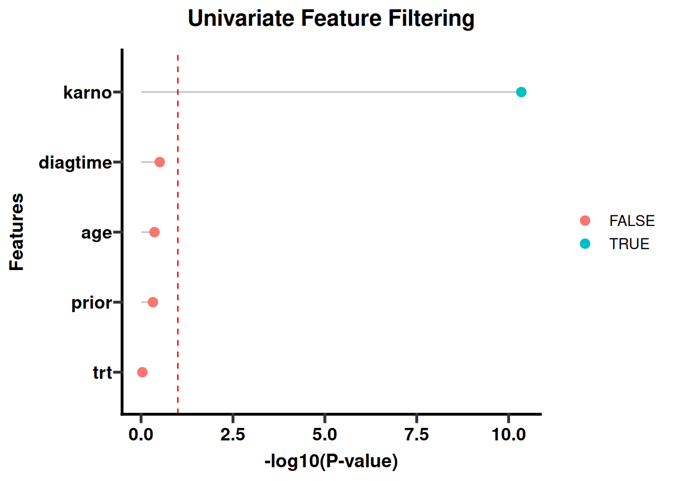
This section selects candidate features. Consider effect size, stability, and biological plausibility rather than a single significance measure.
````{r}
#| label: module4-quickstart-04
#| cache: false
#| echo: true
#| message: false
#| warning: false
#| fig-show: hold
#| out-width: '100%'
# 2. Feature Selection (Univariate + LASSO)
# ---------------------------------------------------------------------------
feat_sel <- surv_feature_selection_multi(
  object = prog,
  methods = c("uni_cox", "lasso"),
  p_threshold = 0.1,
  combine = "union",
  verbose = TRUE
)
selected_feats <- feat_sel$selected
cat("Selected features:", paste(selected_feats, collapse = ", "), "\n")
# Store selected features in the PrognosiX object
prog@survival.var <- list(selected = selected_feats)

# ---------------------------------------------------------------------------
````
### 3 Train/Validation Split
This section creates training and validation sets. Restrict feature selection and parameter estimation to the training set to prevent leakage.
````{r}
#| label: module4-quickstart-05
#| cache: false
#| echo: true
#| message: false
#| warning: false
#| fig-show: hold
#| out-width: '100%'
# 3. Train/Validation Split
# ---------------------------------------------------------------------------
task_full <- surv_extract_task(prog)$select(selected_feats)
n <- task_full$nrow
train_idx <- sample(n, floor(0.7 * n))
val_idx   <- setdiff(seq_len(n), train_idx)

train_task <- task_full$clone()$filter(train_idx)
val_task   <- task_full$clone()$filter(val_idx)

# ---------------------------------------------------------------------------
````
### 4 Train a Survival Random Forest
This section trains and compares candidate models. Select models using discrimination, calibration, stability, and clinical utility together.
````{r}
#| label: module4-quickstart-06
#| cache: false
#| echo: true
#| message: false
#| warning: false
#| fig-show: hold
#| out-width: '100%'
# 4. Train a Survival Random Forest
# ---------------------------------------------------------------------------
learner <- surv_get_learner("surv.ranger", train_task)
learner$train(train_task)

# ---------------------------------------------------------------------------
````
### 5 Evaluate on Validation Set
This section performs the core analysis for this stage. Review the output immediately below the code and confirm that data ranges, assumptions, and results match the study design.
````{r}
#| label: module4-quickstart-07
#| cache: false
#| echo: true
#| message: false
#| warning: false
#| fig-show: hold
#| out-width: '100%'
# 5. Evaluate on Validation Set
# ---------------------------------------------------------------------------
# Apparent (training) performance
train_perf <- surv_evaluate_model(learner, train_task)
cat("Training C-index:", round(train_perf$surv.cindex, 4), "\n")
# Validation performance
val_pred <- learner$predict(val_task)
val_cindex <- val_pred$score(msr("surv.cindex"))
cat("Validation C-index:", round(val_cindex, 4), "\n")
# ---------------------------------------------------------------------------
````
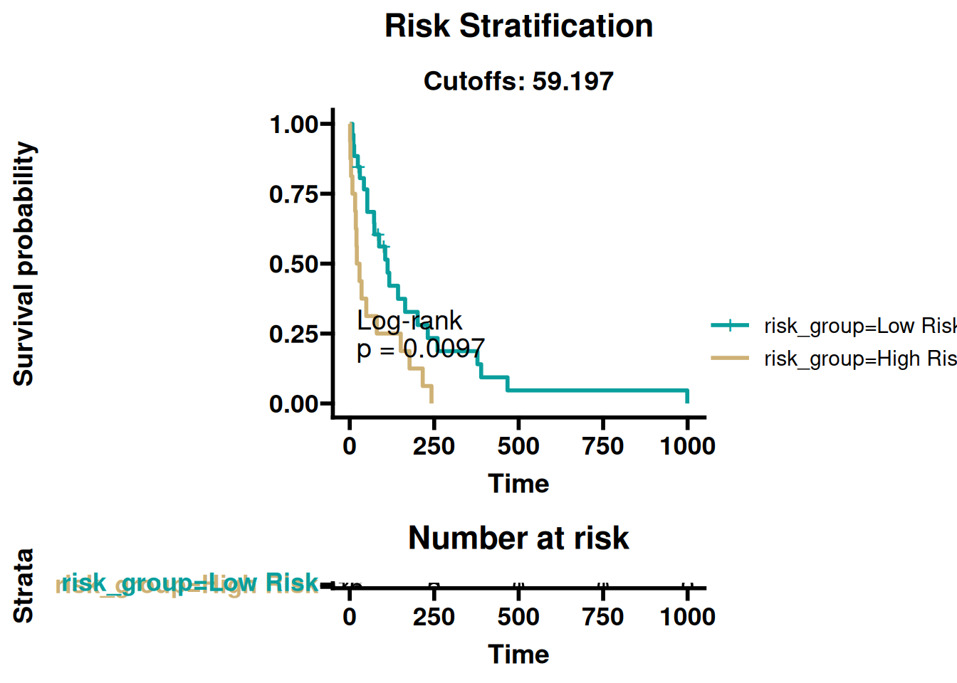
### 6 Risk Stratification and Kaplan‑Meier Plot
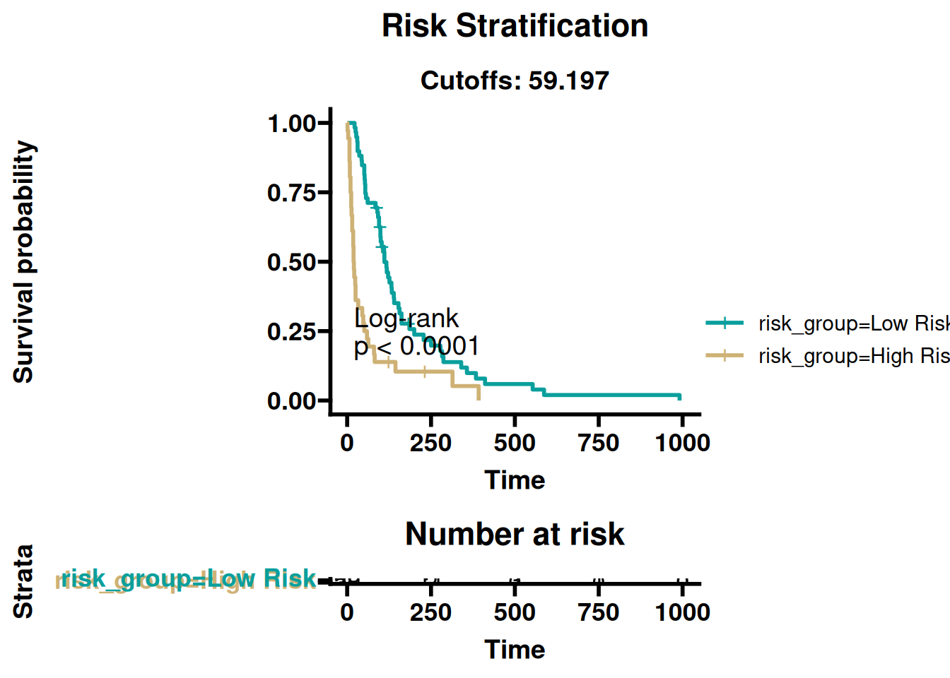
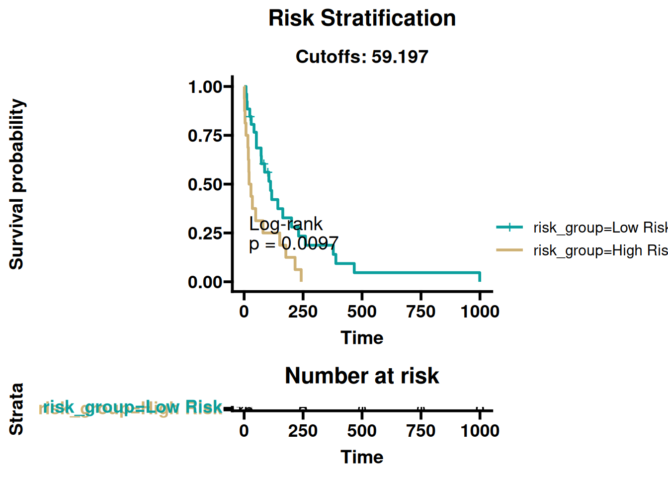
This section creates exploratory and reporting figures. Plots appear below the code and are also saved as vector PDFs for publication.
````{r}
#| label: module4-quickstart-08
#| cache: false
#| echo: true
#| message: false
#| warning: false
#| fig-show: hold
#| out-width: '100%'
# 6. Risk Stratification and Kaplan‑Meier Plot
# ---------------------------------------------------------------------------
# Determine optimal cutoff from training set
pred_train <- learner$predict(train_task)
cut_df <- as.data.frame(train_task$data())
cut_df$risk <- pred_train$crank
cutoff <- median(cut_df$risk, na.rm = TRUE)

# Plot KM curves on the training set (median split)
km_median <- surv_plot_risk_km(learner, train_task, "median", risk_table = TRUE)
print(km_median)

# Apply the same cutoff to the validation set
km_val <- surv_plot_risk_km(learner, val_task,
                            cutoff_method = "custom",
                            custom_cutoffs = cutoff,
                            risk_table = TRUE)
print(km_val)

# Save KM plots
print(km_median)


print(km_val)


# ---------------------------------------------------------------------------
````
### 7 Predict Risk for New Patients
This section applies the trained object to new samples. Validate input format, performance, and target population in an independent cohort before deployment.
````{r}
#| label: module4-quickstart-09
#| cache: false
#| echo: true
#| message: false
#| warning: false
#| fig-show: hold
#| out-width: '100%'
# 7. Predict Risk for New Patients
# ---------------------------------------------------------------------------
# Store the best model in prog@best.model for deployment
prog@best.model <- list(
  learner_id = "surv.ranger",
  learner = learner,
  features = selected_feats,
  cutoff = cutoff,
  decision_type = "binary",
  train_cols = train_task$feature_names
)

# Example new patient data
new_patients <- data.frame(
  celltype = c("smallcell", "adeno"),
  karno    = c(60, 80),
  diagtime = c(10, 5),
  row.names = c("patient_1", "patient_2")
)

risk_scores <- predict_prognosix(prog, new_patients, impute = TRUE)
pred_groups <- predict_risk_groups(prog, new_patients,
                                   cutoff_method = "median",
                                   return_scores = TRUE)

cat("Risk scores:\n"); print(risk_scores)
cat("Risk groups:\n"); print(pred_groups)
# ---------------------------------------------------------------------------
````
### 8 Save the Model
This section trains and compares candidate models. Select models using discrimination, calibration, stability, and clinical utility together.
````{r}
#| label: module4-quickstart-10
#| cache: false
#| echo: true
#| message: false
#| warning: false
#| fig-show: hold
#| out-width: '100%'
# 8. Save the Model
# ---------------------------------------------------------------------------
saveRDS(prog, file = file.path(OUTPUT_DIR, "prog_obj_quickstart.rds"))

cat("\n========================================\n")
cat("Quick‑start pipeline completed successfully!\n")
cat("Validation C-index:", round(val_cindex, 4), "\n")
cat("Results saved in:", OUTPUT_DIR, "\n")
cat("========================================\n")
````