# Module 3: Unsupervised Subtyping — Quick Start
This chapter converts `stat_obj.rds` into icare's `Subtyping` object and uses non-negative matrix factorization (NMF) to discover and visualize candidate patient subtypes. Unlike a purely descriptive clustering result, the fitted NMF model can be retained and applied to new samples after the original preprocessing has been replayed.
## Important Notes
NMF requires non-negative numeric features. Exclude identifiers and known outcomes from the feature matrix, supply the correct group/ID columns to normalization, and verify that all remaining inputs are numeric. Interpret the number and meaning of subtypes with stability, external validation, and clinical relevance—not visualization alone.
## Step-by-step Workflow
<!-- split-into-step-chunks -->
The workflow is divided into short stages. Each note explains the purpose, key checks, and interpretation limits. Generated plots and tables appear directly below their code chunk.
### Environment and Global Setup
This section performs the core analysis for this stage. Review the output immediately below the code and confirm that data ranges, assumptions, and results match the study design.
````{r}
#| label: module3-quickstart-01
#| cache: false
#| echo: true
#| message: false
#| warning: false
#| fig-show: hold
#| out-width: '100%'
# =============================================================================
# icare Package Vignette — Module 3: Subtyping / Unsupervised Clustering
# QUICK-START EDITION
# =============================================================================
# Audience : Users who just want to find and visualize subtypes in their
#            data without comparing every clustering algorithm.
# Input    : "stat_obj.rds", produced by Module 1 (data cleaning).
#
# This script uses NMF as the single clustering method, since it also
# produces a re-usable model for classifying new samples later.
#
# Looking for K-means/LPA comparisons, cluster validation, marker-feature
# heatmaps, or a deployment app? See "03_module3_subtyping_ADVANCED.R".
# =============================================================================

library(icare)
library(NMF)

set.seed(123)

# ---------------------------------------------------------------------------
````
### 1 Load the cleaned data and convert it into a Subtyping object
This section imports and organizes the data. Check dimensions and variable coding before continuing.
````{r}
#| label: module3-quickstart-02
#| echo: true
#| message: false
#| warning: false
#| fig-show: hold
#| out-width: '100%'
# 1. Load the cleaned data and convert it into a Subtyping object
# ---------------------------------------------------------------------------
stat_obj <- readRDS("stat_obj.rds")
sub_obj  <- ConvertObject(stat_obj, to = "Subtyping")
# min-max scaling: NMF requires non-negative input.
# IMPORTANT: pass the ACTUAL name of your outcome/ID column via `group_col`
# (default is "group") -- Sub_normalize_process() only excludes a column
# from scaling by an EXACT name match, and it never removes non-numeric
# columns from what it returns. If group_col doesn't match your real column
# name, or clean.data has any other non-numeric column (site, ID, free
# text...), it will silently survive into scale.data and later crash NMF
# deep inside with an unrelated-looking "'x' must be numeric" error.
# Replace "group" below with your real outcome column name if different.
features=colnames(sub_obj@scale.data)[colnames(sub_obj@scale.data)!='sex']
sub_obj@clean.data <- sub_obj@clean.data[, features, drop = FALSE]
sub_obj <- Sub_normalize_process(sub_obj, normalize_method = "min_max",
                                 group_col = "group")
# Defensive check BEFORE clustering: make sure every remaining column is
# actually numeric. If this stops, the message tells you exactly which
# column(s) to exclude or fix group_col for.
non_numeric_cols <- names(sub_obj@scale.data)[!vapply(sub_obj@scale.data, is.numeric, logical(1))]
if (length(non_numeric_cols) > 0) {
  stop("Non-numeric column(s) in scale.data: ", paste(non_numeric_cols, collapse = ", "),
       ". Set group_col correctly above, or drop these columns from ",
       "clean.data before calling Sub_normalize_process().")
}

# Drop zero-variance columns (they can break the clustering step).
sub_obj@scale.data <- remove_constant_columns(sub_obj@scale.data)
# ---------------------------------------------------------------------------
````
### 2 Estimate the number of subtypes, then cluster
This section performs the core analysis for this stage. Review the output immediately below the code and confirm that data ranges, assumptions, and results match the study design.
````{r}
#| label: module3-quickstart-03
#| echo: true
#| message: false
#| warning: false
#| fig-show: hold
#| out-width: '100%'
# 2. Estimate the number of subtypes, then cluster
# ---------------------------------------------------------------------------
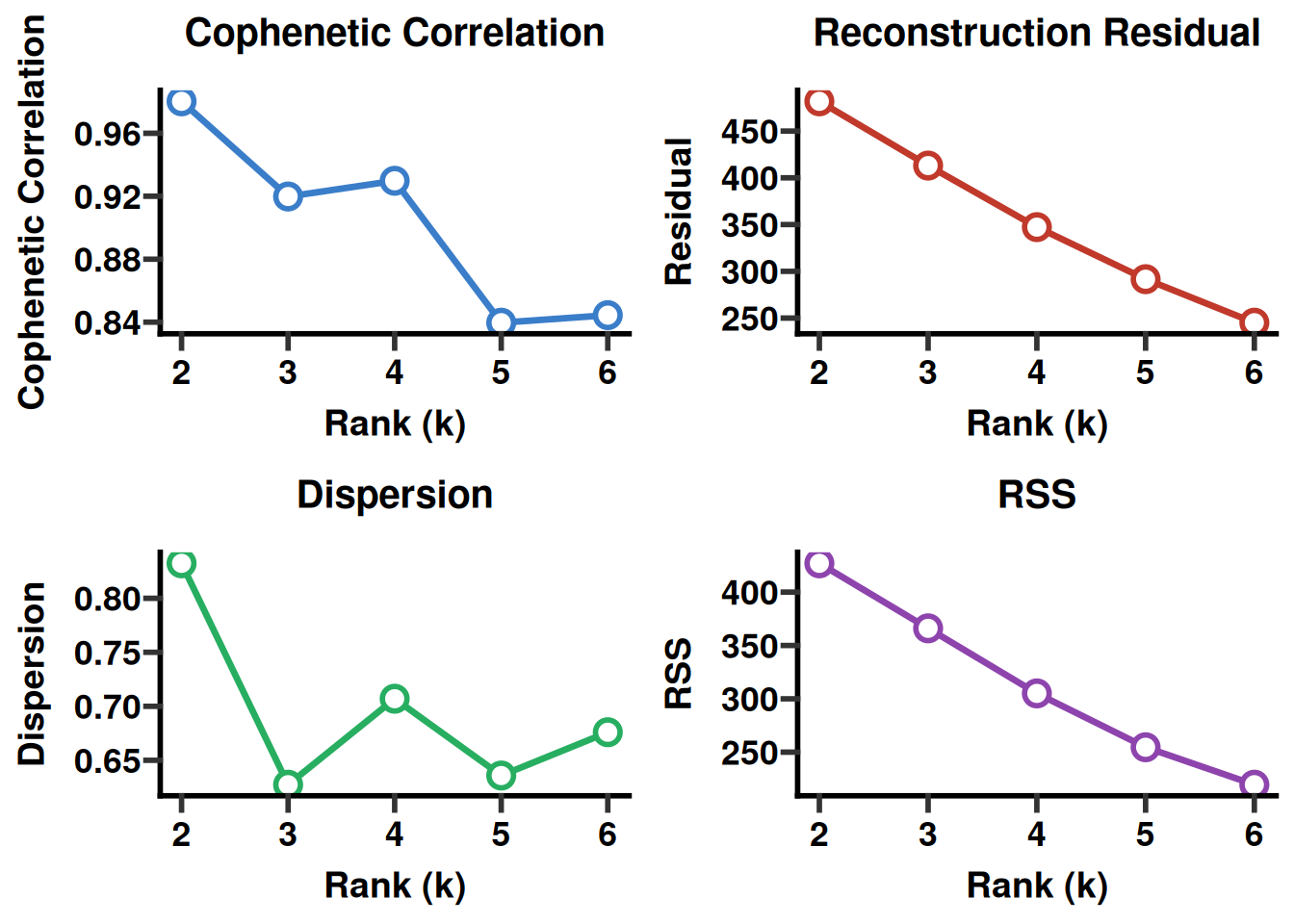
sub_obj <- Sub_nmf_estimate(sub_obj, rank_range = 2:6, nrun = 5, method = "brunet")
sub_obj <- Sub_nmf_best_rank(sub_obj, nrun = 5, method = "brunet")
cat("Optimal number of subtypes:", sub_obj@Optimal.cluster, "\n")
sub_obj <- Sub_nmf_assign_subtypes(sub_obj)
print(table(sub_obj@info.data$cluster_nmf))
# ---------------------------------------------------------------------------
````
### 3 Visualize the subtypes
This section creates exploratory and reporting figures. Plots appear below the code and are also saved as vector PDFs for publication.
````{r}
#| label: module3-quickstart-04
#| echo: true
#| message: false
#| warning: false
#| fig-show: hold
#| out-width: '100%'
# 3. Visualize the subtypes
# ---------------------------------------------------------------------------
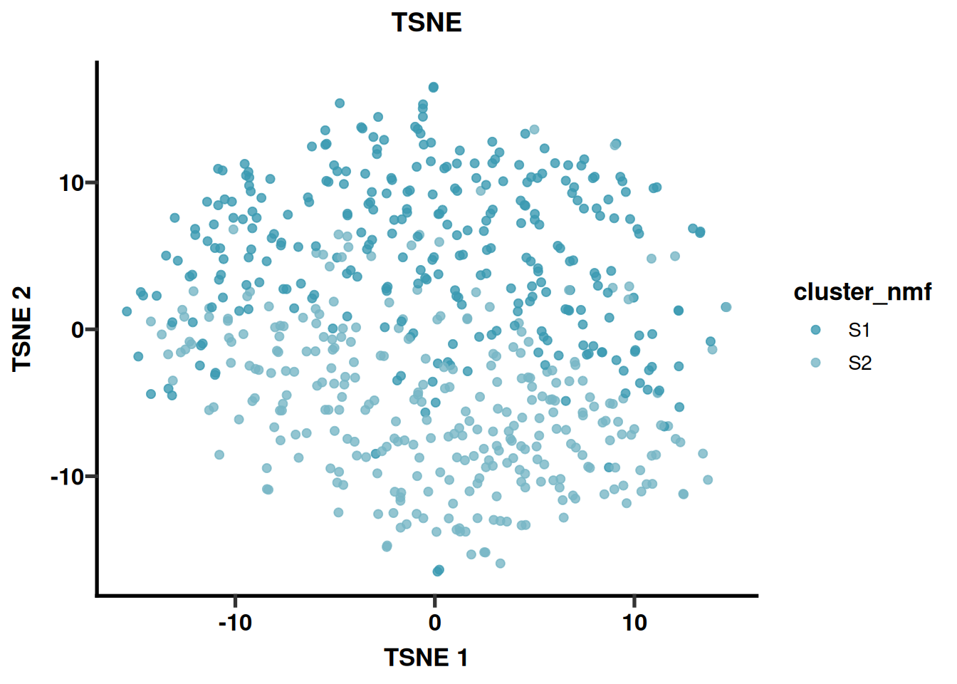
sub_obj <- Sub_tsne_analyse(sub_obj, use_scaled_data = TRUE)
PlotDimReduction(sub_obj, reduction = "tsne", color_by = "cluster_nmf",
                 palette_name = "Zissou1", save_plot = TRUE)
# ---------------------------------------------------------------------------
````
### 4 Check cluster quality and find marker features
This section evaluates quality and robustness. Interpret plots, metrics, and sample distributions together.
````{r}
#| label: module3-quickstart-05
#| echo: true
#| message: false
#| warning: false
#| fig-show: hold
#| out-width: '100%'
# 4. Check cluster quality and find marker features
# ---------------------------------------------------------------------------
sub_obj@clustered.data$group <- sub_obj@info.data$cluster_nmf
eval_result <- Sub_evaluation_results(sub_obj, seed = 123)
print(eval_result@evaluation_results)
deg_df <- sub_obj@clean.data
deg_df$subtype <- factor(sub_obj@info.data$cluster_nmf)
multi_deg <- batch_Wilcoxon_MultiClass(mat = deg_df, group_col = "subtype", only.pos = FALSE)

tryCatch(
  PlotClusterHeatmap(
    sub_obj, p_cutoff = 2, deg_df = multi_deg, top_n = 5,
    group_by = "cluster_nmf", save_path = "./subtype_marker_heatmap.pdf"
  ),
  error = function(e) message(
    "Sample-level subtype heatmap skipped because the macOS raster backend ",
    "could not create its temporary image: ", e$message
  )
)

# ---------------------------------------------------------------------------
````
### 5 Save your results
This section saves model objects, tables, and figures for reproducibility, review, and reuse.
````{r}
#| label: module3-quickstart-06
#| echo: true
#| message: false
#| warning: false
#| fig-show: hold
#| out-width: '100%'
# 5. Save your results
# ---------------------------------------------------------------------------
saveRDS(sub_obj, file = "subtyping_obj.rds")

cat("\nDone! subtyping_obj.rds saved.\n",
    "Want to compare K-means/LPA, validate clusters more thoroughly,",
    "or deploy a prediction app? See the ADVANCED version of this script.\n")
````