# Module 1: Data Cleaning and Exploration — Advanced
The advanced `Stat` workflow covers raw-data diagnostics, automatic and manual type handling, missing-value imputation, outlier treatment, one-hot encoding, normalization, grouped plots, correlation heatmaps, PCA, differential features, ROC analysis, radar plots, and Table 1. Together, these steps implement the package's clinical-statistics and exploratory-analysis layer before downstream prediction or subtyping.
## Key Configuration
Set `GROUP_COL`, `OUTPUT_DIR`, and `N_TOP_FEATURES` in the `CONFIG` section. Review every inferred data type and retain a record of imputation and scaling decisions. Outputs are organized into subdirectories so that quality-control results, statistical summaries, and publication figures can be audited separately.
## Step-by-step Workflow
The workflow is divided into short stages. Each note explains the purpose, key checks, and interpretation limits. Generated plots and tables appear directly below their code chunk.
### About this chapter
**Audience.** Advanced users preparing figures and tables for a manuscript, or anyone who wants to see every configurable option in the Module 1 pipeline.
**Input.** Reads `data/PMID37633276_DIA_plasmaproomic.xlsx` (sheet 3) directly.
The chapter runs end to end as one session:
1. **CONFIG — the only section you should need to edit for a new dataset**
2. **Load Data**
3. **Create the Stat Object**
4. **Pre-cleaning Exploratory Analysis**
5. **Data Cleaning Pipeline**
6. **Publication-Quality Visualizations**
7. **Additional Descriptive Visualizations**
8. **Differential Feature Analysis (Wilcoxon Test)**
9. **Differential-Feature Visualizations**
10. **Reporting & Result Export**
### 0 CONFIG — the only section you should need to edit for a new dataset
This section defines seeds, output paths, and dependencies. Update these paths and key parameters first when using new data.
````{r}
#| label: module1-advanced-09
#| echo: true
#| message: false
#| warning: false
#| fig-show: hold
#| out-width: '100%'
# 0. CONFIG — the only section you should need to edit for a new dataset
# ---------------------------------------------------------------------------
options(warn = -1)
rm(list = ls())
library(icare)

GROUP_COL  <- "group"                              # outcome / group column
OUTPUT_DIR <- "./Module1_Advanced_Output"                  # all figures/tables go here
N_TOP_FEATURES <- 10                                       # how many DEGs to carry into plots

dir.create(OUTPUT_DIR, showWarnings = FALSE, recursive = TRUE)
# Register OUTPUT_DIR with the package rather than defining a local sub_dir().
# icare already ships sub_dir(); a local definition shadows it only inside this
# script, so functions INSIDE the package that call sub_dir() themselves would
# still resolve it in the icare namespace and write somewhere else. Calling
# set_output_root() points both this script and the package at the same tree.
set_output_root(OUTPUT_DIR)

# =============================================================================
````
### 1 Load Data
This section imports and organizes the data. Check dimensions and variable coding before continuing.
````{r}
#| label: module1-advanced-10
#| echo: true
#| message: false
#| warning: false
#| fig-show: hold
#| out-width: '100%'
# 1. Load Data
# =============================================================================
# stringsAsFactors = FALSE keeps everything as character/numeric for now;
library(readxl)
raw_dis=as.data.frame(read_excel("data/PMID37633276_DIA_plasmaproomic.xlsx",sheet = 3))
raw_dis=raw_dis[!grepl(x = raw_dis$`Case ID`,pattern = "^KC"),]
dput(colnames(raw_dis))
mat=raw_dis[,c( "White blood cell count",
                "Lymphocytes%", "Monocytes%", "Neutrophilic granulocyte%", "Eosinophil%",
                "Basophil%", "Lymphocytes count", "Monocytes count", "Neutrophilic granulocyte count",
                "Eosinophil count", "Basophil count", "Red blood cell count",
                "Hemoglobin", "Hematocrit", "Mean red blood cell volume", "Mean cell hemoglobin",
                "Mean corpuscular hemoglobin concentration", "Red blood cell distribution width CV",
                "Red blood cell distribution width SD", "Platelet count", "Mean platelet volume",
                "PCT", "Platelet volume distribution width")]
index=grepl(x = raw_dis$`Case ID`,pattern = "^HC")
inf=raw_dis[,c("Case ID", "Sample type", "Plasma proteome ID", "Tissue proteome ID",
               "Gender", "Age at diagnosis", "Tobacco smoking history", "Drinking history",
               "Vital status", "Days to last followup", "Days until death",
               "Combined days to last followup or death", "Progressive-free survival_Status",
               "Progressive-free survival_Months", "Tumor location", "Tumor size (cm)",
               "T-category", "Lymph node involvement", "Distant metastasis",
               "TNM Stage", "Grade", "Morphology")]
# The group label goes in `inf` ONLY. icare stores the label in info.data and
# keeps it out of the feature matrix entirely: a label sitting among the
# features is indistinguishable from a feature to any code that selects columns
# by type, and a numeric 0/1 label would silently be fed into PCA and the
# correlation heatmap. Because the label never enters `mat`, its R type is free
# -- labels can be readable strings, which is what you want in the Table 1
# column headers.
inf$group = factor(ifelse(index, "Healthy Control", "Case"),
                   levels = c("Healthy Control", "Case"))

# `mat` stays purely numeric, so as.matrix()/storage.mode() is a safe no-op and
# any non-numeric column here would be a genuine mistake rather than a silent NA.
mat=as.matrix(mat)
storage.mode(mat) <- "numeric"

rownames(mat)=inf$`Case ID`
rownames(inf)=inf$`Case ID`
mat=as.data.frame(mat)
mat$age=inf$`Age at diagnosis`
mat$sex=inf$Gender
# =============================================================================
````
### 2 Create the Stat Object
This section creates the icare analysis object that stores data, metadata, and workflow state for all later steps.
````{r}
#| label: module1-advanced-11
#| echo: true
#| message: false
#| warning: false
#| fig-show: hold
#| out-width: '100%'
# 2. Create the Stat Object
# =============================================================================
# CreateStatObject() is the entry point of icare: it stores the raw data,
# remembers which column is the grouping/outcome variable, and will
# accumulate every cleaning step you apply to it (accessible via
# stat_obj@clean.data once cleaning is done).
# na.action = "allow" means missing values are kept for now; we handle them
# explicitly in the cleaning section (step 4.2) rather than dropping rows here.
stat_obj <- CreateStatObject(
  raw.data  = mat,info.data = inf,
  group_col = "group",
  na.action = "allow"
)
cat("Stat object created.\n")
# =============================================================================
````
### 3 Pre-cleaning Exploratory Analysis
This section preprocesses the data. Review missingness, outlier handling, and normalization before accepting the defaults.
````{r}
#| label: module1-advanced-12
#| echo: true
#| message: false
#| warning: false
#| fig-show: hold
#| out-width: '100%'
# 3. Pre-cleaning Exploratory Analysis
# =============================================================================
## 3.1 Missing-data visualization — shows which variables/rows are most
##     affected, which should guide your imputation strategy in step 4.2
stat_obj <- state_plot_missing_data(
  stat_obj,
  save_plots = TRUE,
  save_data  = TRUE,
  save_dir   = sub_dir("01_exploration", "missing_data")
)
## 3.2 Variable type diagnosis — auto-detects numeric vs. categorical columns.
## max_unique_values = 5 means any column with <= 5 unique values is treated
## as categorical even if it is stored as numbers (e.g. a 0/1/2 coded score).
stat_obj <- stat_diagnose_variable_type(stat_obj, max_unique_values = 5)
cat("Detected variable types:\n"); print(stat_obj@variable.types)
## 3.3 Descriptive statistics on the RAW data, before any cleaning.
## Keeping a "before" summary alongside the "after" one (produced later) is
## good practice for a methods section: it lets you report what changed.
stat_obj <- stat_compute_descriptive(stat_obj, count_feature = TRUE)
# =============================================================================
````
### 4 Data Cleaning Pipeline
This section preprocesses the data. Review missingness, outlier handling, and normalization before accepting the defaults.
````{r}
#| label: module1-advanced-13
#| echo: true
#| message: false
#| warning: false
#| fig-show: hold
#| out-width: '100%'
# 4. Data Cleaning Pipeline
# =============================================================================
## 4.1 Convert columns to their diagnosed types (numeric / factor)
stat_obj <- stat_convert_variables(stat_obj, save_data = FALSE)
## 4.2 Impute missing values.
## "median_mode" = median for numeric columns, mode for categorical ones —
## a simple, fast, and reasonably robust default. For datasets with more
## complex/structured missingness, consider impute_method = "mice" instead
## (see the alternative Module 1 script for a worked example).
stat_obj <- stat_miss_processed(
  stat_obj,
  impute_method = "mice",
  return_imputation_info = TRUE,
  save_data = FALSE
)
## 4.3 Detect outliers using the IQR rule (values beyond 1.5x the
## interquartile range from Q1/Q3 are flagged, the usual Tukey convention).
stat_obj <- stat_detect_and_mark_outliers(
  stat_obj,
  method    = "iqr",
  threshold = 1.5,
  save_data = FALSE
)
## 4.4 Handle the flagged outliers by replacing them with the column median
## rather than deleting rows, so no samples are lost.
stat_obj <- stat_handle_outliers(
  stat_obj,
  method       = "impute",
  impute_value = "median",
  save_data    = FALSE
)
## 4.5 One-hot encode categorical variables that have more than 2 levels
## (binary variables are left as single 0/1 columns to avoid redundancy).
stat_obj <- stat_onehot_encode(stat_obj, save_data = FALSE)
## 4.6 Normalize numeric features. method = "auto" lets icare pick an
## appropriate transform per-column (e.g. z-score vs. a skew-correcting
## transform) based on each variable's distribution.
stat_obj <- stat_normalize_process(stat_obj, method = "auto", save_data = FALSE)
cat("\nCleaning completed. Clean data dimensions:",
    nrow(stat_obj@clean.data), "x", ncol(stat_obj@clean.data), "\n")
# =============================================================================
````
### 5 Publication-Quality Visualizations
This section creates exploratory and reporting figures. Plots appear below the code and are also saved as vector PDFs for publication.
````{r}
#| label: module1-advanced-14
#| echo: true
#| message: false
#| warning: false
#| fig-show: hold
#| out-width: '100%'
# 5. Publication-Quality Visualizations
# =============================================================================
viz_dir <- sub_dir("02_visualizations")

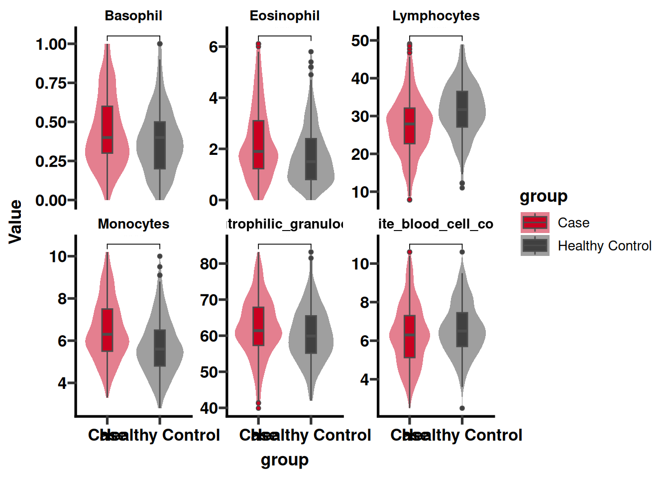
## 5.1 Grouped box + violin plots for the first 6 numeric variables, each
## annotated with a Wilcoxon test p-value between groups. Swap `features`
## for any variable list you want to feature in a figure.
numeric_vars <- names(stat_obj@clean.data)[sapply(stat_obj@clean.data, is.numeric)]
# Key these by the label text, not by a code: the group column holds
# "Healthy Control"/"Case", and unmatched keys would silently fall back.
my_colors <- c("Healthy Control" = "#404040", "Case" = "#ca0020")
PlotGroupedDistribution(
  object       = stat_obj,
  features     = head(numeric_vars, 6),
  group_col    = "group",
  group_colors = my_colors,
  test         = "wilcox.test",
  palette_name = "Set1", height = 8,width = 10,
  ncol         = 3,
  save_dir     = viz_dir,
  save_plot    = TRUE
)
unique(stat_obj@clean.data$group)
## 5.2 Correlation heatmap for a clinically meaningful feature panel
## (here: red-cell indices). Replace `features` with your variables of interest.
PlotCorrelationHeatmap(
  object       = stat_obj,insig = "blank",pch = 3,
  features     = numeric_vars[-24],
  color_scheme = "gradient",   # alternative: "brew"
  save_dir     = viz_dir,
  save_plot    = TRUE
)
## 5.3 PCA scatter plot coloured by the outcome group, with 95% confidence
## ellipses — a standard "does the outcome separate along the main axes of
## variation" sanity check before modeling.
# Key these by the label text, not by a code: the group column holds
# "Healthy Control"/"Case", and unmatched keys would silently fall back.
my_colors <- c("Healthy Control" = "#404040", "Case" = "#ca0020")
PlotPCA(
  object       = stat_obj,
  color_by     = "group",
  group_colors = my_colors,
  pcs          = c(1, 2),
  ellipse      = TRUE,
  palette_name = "Royal1",
  save_dir     = viz_dir,
  save_plot    = TRUE
)
# =============================================================================
````
### 6 Additional Descriptive Visualizations
This section creates exploratory and reporting figures. Plots appear below the code and are also saved as vector PDFs for publication.
````{r}
#| label: module1-advanced-15
#| echo: true
#| message: false
#| warning: false
#| fig-show: hold
#| out-width: '100%'
# 6. Additional Descriptive Visualizations
# =============================================================================
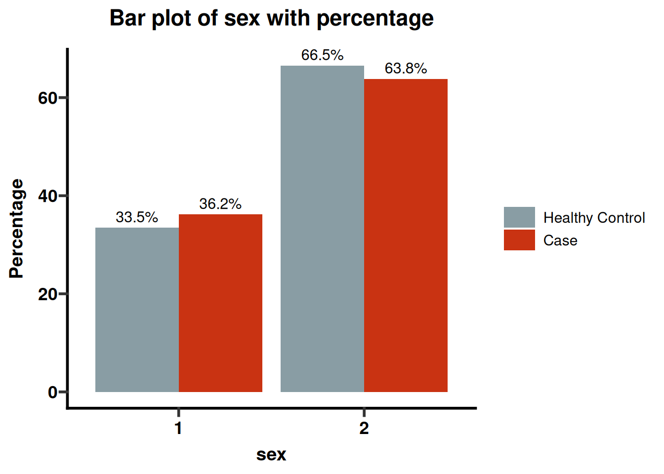
## 6.1 Bar plots for every categorical variable
stat_obj <- plot_categorical_descriptive(stat_obj, save_plots = TRUE, save_dir = viz_dir)
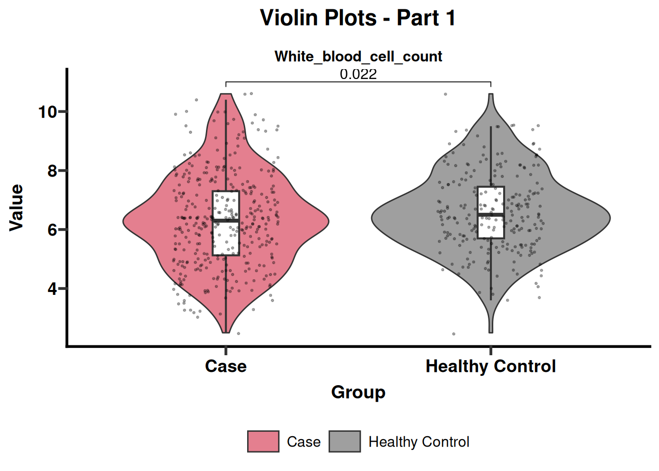
## 6.2 Violin plots for every numeric variable (one plot per variable)
# Key these by the label text, not by a code: the group column holds
# "Healthy Control"/"Case", and unmatched keys would silently fall back.
my_colors <- c("Healthy Control" = "#404040", "Case" = "#ca0020")
stat_obj <- plot_numeric_descriptive(
  stat_obj, plot_type = "violin", vars_per_plot = 1,group_col = 'group',group_colors = my_colors,
  save_plots = TRUE, save_dir = viz_dir
)
## 6.3 Ridge (density) plots — an alternative view of the same numeric
## variables, useful when distributions are multi-modal.
library(ggridges)
stat_obj <- plot_numeric_descriptive(
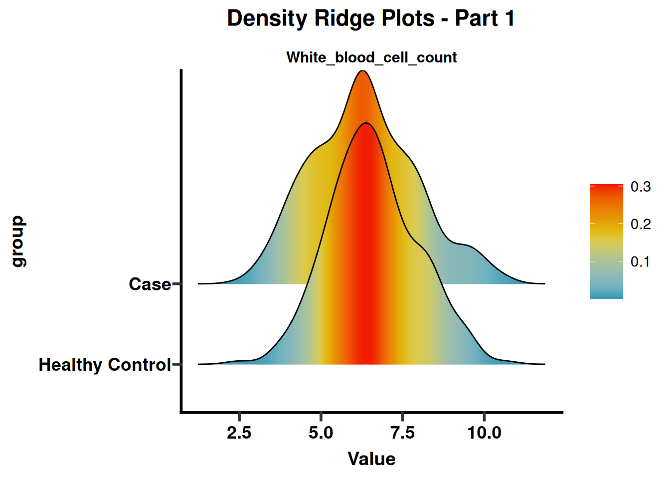
  stat_obj, plot_type = "ridge", vars_per_plot = 1,
  save_plots = TRUE, save_dir = viz_dir
)
# =============================================================================
````
### 7 Differential Feature Analysis (Wilcoxon Test)
This section selects candidate features. Consider effect size, stability, and biological plausibility rather than a single significance measure.
````{r}
#| label: module1-advanced-16
#| echo: true
#| message: false
#| warning: false
#| fig-show: hold
#| out-width: '100%'
# 7. Differential Feature Analysis (Wilcoxon Test)
# =============================================================================
deg_dir <- sub_dir("03_differential_analysis")
stat_obj <- stat_var_feature(stat_obj, p_threshold = 0.05, logfc_threshold = 0.1,save_data = TRUE)
deg_result <- ExtractLastTestSig(stat_obj)
# Standardize the "feature name" column (some downstream plotting functions
# expect a column literally called `feature`).
deg_result$feature <- deg_result$id

# Rank features by adjusted p-value and keep the top N for downstream plots —
# this replaces any ad hoc/undefined feature list with an explicit, reproducible one.
top_ids <- head(deg_result$id[order(deg_result$p.adjust)], N_TOP_FEATURES)

# =============================================================================
````
### 8 Differential-Feature Visualizations
This section selects candidate features. Consider effect size, stability, and biological plausibility rather than a single significance measure.
````{r}
#| label: module1-advanced-17
#| echo: true
#| message: false
#| warning: false
#| fig-show: hold
#| out-width: '100%'
# 8. Differential-Feature Visualizations
# =============================================================================
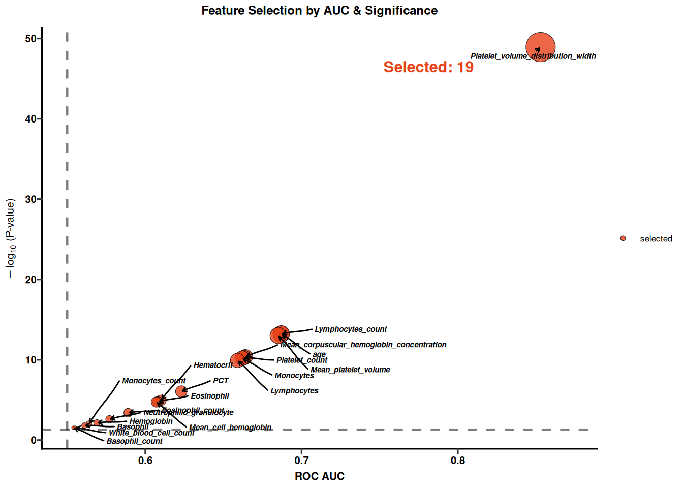
## 8.1 AUC vs. p-value scatter — flags features that are both statistically
## significant AND discriminative (AUC far from 0.5).
PlotAUCPval(
  deg_df     = deg_result,
  # PlotAUCPval() takes a plain data frame and expects the label alongside the
  # features. Since Stat@clean.data is label-free by contract, join it back from
  # info.data for this call (the public helper .stat_with_group does exactly this).
  mat_test   = icare:::.stat_with_group(stat_obj),
  group_col  = GROUP_COL,base_size = 8,text_repel_size = 2,
  auc_thresh = 0.55,
  p_thresh   = 0.05,
  save_dir   = deg_dir,
  save_plot  = TRUE
)
## 8.2 Heatmap of the top differential features across samples
# Build the top annotation (assuming rownames(mat) contains sample IDs)
top_anno <- stat_obj@info.data
# info.data column names are normalised by CreateStatObject() (spaces become
# underscores), so reference the normalised names, not the original Excel header.
top_anno <-top_anno [,c('Gender','Age_at_diagnosis')]
# Custom color palette
custom_cols <- list(
  group= c("Case" = "#404040", "Healthy Control" = "#ca0020"),
  Gender= c( Female= "#018571", Male = "#a6611a"),
  `Age_at_diagnosis`= circlize::colorRamp2(c(40, 55, 70), c("#edf8b1", "#7fcdbb", "#2c7fb8"))
)
PlotFeatureHeatmap(
  object = stat_obj,
  features = top_ids,
  top_annotation = top_anno,
  ann_colors = custom_cols,
  cluster_rows   = TRUE,
  show_rownames  = TRUE,
  save_dir       = deg_dir,
  color_palette = c("lightgray", "#7B1FA2", "black", "gold") ,
  save_plot      = TRUE
)
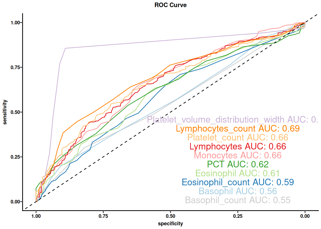
## 8.3 ROC curves for the top differential features (per-feature discrimination)
library(pROC)
stat_obj <- VarFeature_ROC(stat_obj, data_type = "clean", save_dir = deg_dir, save_plots = TRUE,
                           palette_name = 'Paired',base_size = 8)
## 8.4 Radar chart summarizing mean expression shifts between groups
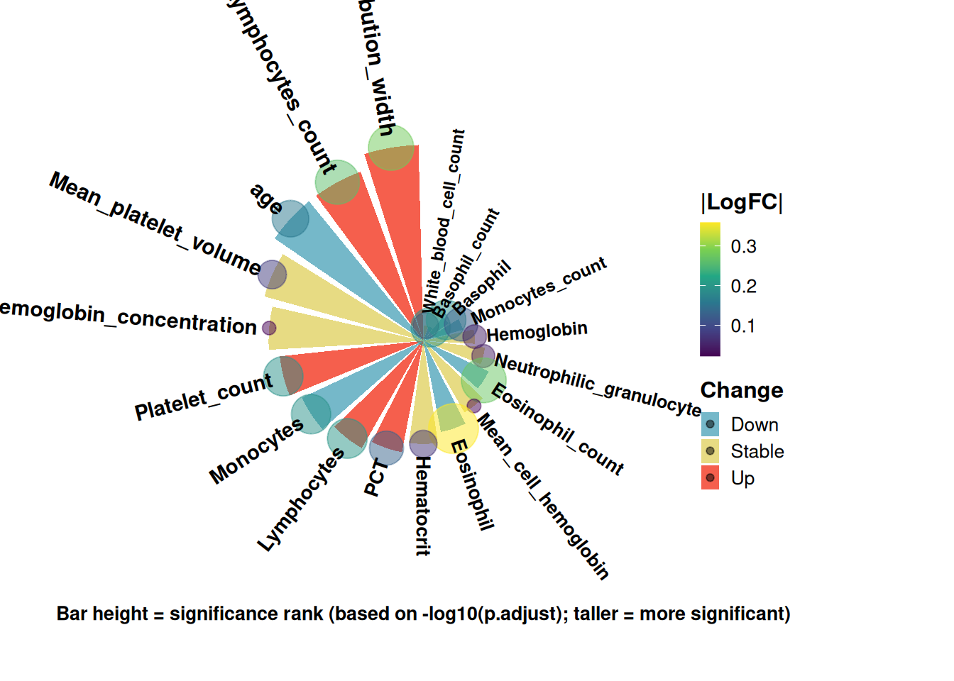
stat_obj <- VarFeature_radarchart(stat_obj, save_dir = deg_dir, save_plots = TRUE,drop_stable = F,base_size = 6,
                                  sort_by = 'pvalue',plot_width = 8,plot_height = 8,title = '')
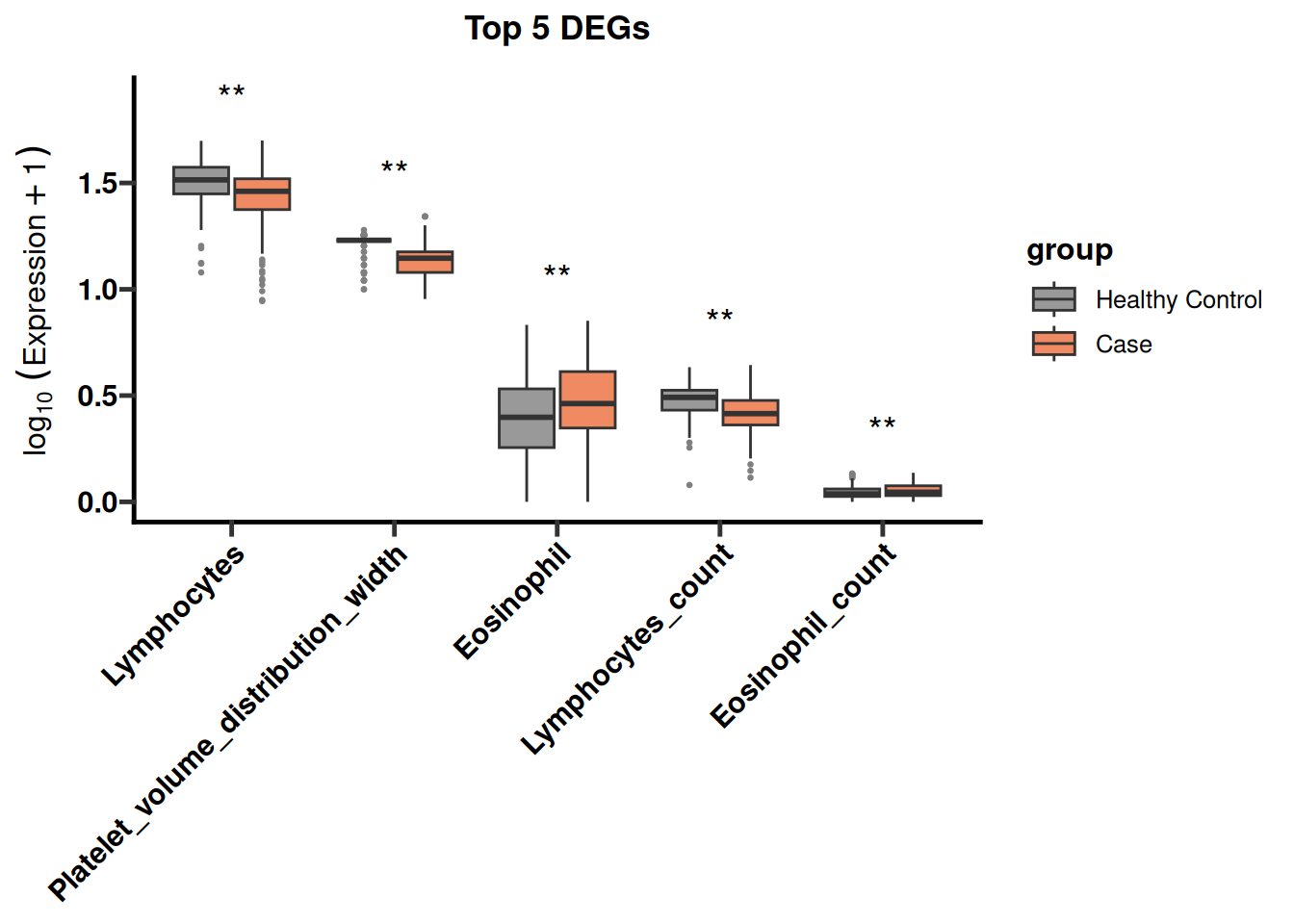
## 8.5 Boxplots for the top 3 differential features (raw/clean scale)
p_box <- PlotDegBoxplot(
  deg_results = deg_result,
  # PlotDegBoxplot() takes a plain data frame and needs the label beside the
  # features; Stat@clean.data is label-free by contract, so join it back.
  expr_data   = icare:::.stat_with_group(stat_obj),
  group_col   = GROUP_COL,
  top_n       = 5,
  save_plot   = TRUE,
  save_dir    = deg_dir
)
# =============================================================================
````
### 9 Reporting & Result Export
This section saves model objects, tables, and figures for reproducibility, review, and reuse.
````{r}
#| label: module1-advanced-18
#| echo: true
#| message: false
#| warning: false
#| fig-show: hold
#| out-width: '100%'
# 9. Reporting & Result Export
# =============================================================================
## 9.1 Baseline characteristics table ("Table 1" for a manuscript), written
## to a Word document for easy copy-paste into a submission.
stat_obj <- stat_gaze_analysis(stat_obj, save_word = TRUE, save_dir = OUTPUT_DIR)
cat("\nBaseline table generated.\n")
if (!is.null(stat_obj@baseline.table)) print(stat_obj@baseline.table)
## 9.2 Sanity check: replay the exact same cleaning pipeline on a fresh
## sample of data, to confirm the pipeline generalizes beyond the training rows.
set.seed(123)
new_data <- mat[sample(seq_len(nrow(mat)), 30), ]
processed_new <- process_new_data(stat_object = stat_obj, new_data = new_data, save_data = FALSE)
cat("\nNew data processed. Dimensions:", nrow(processed_new), "x", ncol(processed_new), "\n")
## 9.3 Extract the final cleaned dataset for use outside icare if needed
final_clean <- ExtractCleanData(stat_obj)
cat("\nFinal clean dataset dimensions:", nrow(final_clean), "x", ncol(final_clean), "\n")
write.csv(final_clean, file.path(OUTPUT_DIR, "clean_data_final.csv"), row.names = FALSE)

## 9.4 Save the Stat object itself — Module 2 (modeling) and Module 3
## (subtyping) both load this file directly via readRDS("stat_obj.rds"),
## so it is intentionally saved at the project root rather than inside
## OUTPUT_DIR.
saveRDS(stat_obj, file = "stat_obj.rds")

cat("\n========================================\n")
cat("Module 1 (advanced) pipeline finished successfully!\n")
cat("All figures/tables saved under:", OUTPUT_DIR, "\n")
cat("========================================\n")
````