# Module 2: Classification Modeling — Quick Start
This chapter converts the cleaned `Stat` object into icare's `Train_Model` object, selects informative features, performs a stratified development split, estimates preprocessing from training data, benchmarks common classifiers through the caret-based interface, and selects a final model using held-out AUC.
## Important Notes
The `Train_Model` object is designed to preserve the modeling state needed for later prediction and deployment. Estimate imputation, scaling, feature selection, tuning, and decision thresholds from training data only, then apply the stored operations unchanged to the test set. Preserve this sequence when changing the data, class outcome, or resampling design.
## Step-by-step Workflow
<!-- split-into-step-chunks -->
The workflow is divided into short stages. Each note explains the purpose, key checks, and interpretation limits. Generated plots and tables appear directly below their code chunk.
### Environment and Global Setup
This section performs the core analysis for this stage. Review the output immediately below the code and confirm that data ranges, assumptions, and results match the study design.
````{r}
#| label: module2-quickstart-01
#| cache: false
#| echo: true
#| message: false
#| warning: false
#| fig-show: hold
#| out-width: '100%'
# =============================================================================
# icare Package Vignette — Module 2: Modeling Pipeline
# QUICK-START EDITION
# =============================================================================
# Audience : Users who just want a trained, evaluated model without exploring
#            every feature-selection method, ensemble strategy, or clinical
#            extra.
# Input    : "stat_obj.rds", produced by Module 1 (data cleaning).
#
# This script covers: convert to a modeling object -> select features ->
# split & scale -> train a few algorithms -> pick the best -> evaluate it.
#
# Looking for feature-selection comparisons, ensembles, tuning, SHAP
# explanations, or clinical thresholds/NRI? See
# "02_module2_modeling_ADVANCED.R" instead.
# =============================================================================
rm(list = ls())
library(icare)
library(caret)

set.seed(123)

# ---------------------------------------------------------------------------
````
### 1 Load the cleaned data and convert it into a modeling object
This section imports and organizes the data. Check dimensions and variable coding before continuing.
````{r}
#| label: module2-quickstart-02
#| echo: true
#| message: false
#| warning: false
#| fig-show: hold
#| out-width: '100%'
# 1. Load the cleaned data and convert it into a modeling object
# ---------------------------------------------------------------------------
stat_obj  <- readRDS("stat_obj.rds")
model_obj <- ConvertObject(stat_obj, to = "Train_Model")
model_obj@clean.df[[model_obj@group_col]] <- factor(model_obj@clean.df[[model_obj@group_col]])

# ---------------------------------------------------------------------------
````
### 2 Quick feature selection (built-in importance from a couple of models)
This section selects candidate features. Consider effect size, stability, and biological plausibility rather than a single significance measure.
````{r}
#| label: module2-quickstart-03
#| echo: true
#| message: false
#| warning: false
#| fig-show: hold
#| out-width: '100%'
# 2. Quick feature selection (built-in importance from a couple of models)
# ---------------------------------------------------------------------------
builtin <- FeatureSelectBuiltin(
  object = model_obj,
  models = c("rf", "glm"),
  top_n  = 15,
  seed   = 123
)
print(builtin$importance_table)
# Keep only the top features identified above.
model_obj <- ApplyFeatureSelection(model_obj,builtin$importance_table$Feature[1:15])
colnames(model_obj@clean.df)
# ---------------------------------------------------------------------------
````
### 3 Split into training/testing sets and scale the predictors
This section creates training and validation sets. Restrict feature selection and parameter estimation to the training set to prevent leakage.
````{r}
#| label: module2-quickstart-04
#| echo: true
#| message: false
#| warning: false
#| fig-show: hold
#| out-width: '100%'
# 3. Split into training/testing sets and scale the predictors
# ---------------------------------------------------------------------------
# Stratified split: create 70% training indices while preserving
#    the distribution of the grouping variable (e.g., response class)
#    using caret's createDataPartition.
#    - model_obj@clean.df: the cleaned data frame
#    - model_obj@group_col: name of the column used for stratification
#    - p = 0.7: proportion for training
#    - list = FALSE: returns a vector of indices instead of a list
idx <- createDataPartition(model_obj@clean.df[[model_obj@group_col]], p = 0.7, list = FALSE)
# Split the original clean data into training and testing sets
#    based on the indices, and store them in the 'split.data' slot
#    of the S4 object.
model_obj@split.data <- list(
  training = model_obj@clean.df[idx, ],
  testing  = model_obj@clean.df[-idx, ]
)
# Compute pre-processing parameters (center and scale) from the
#    training set, but ONLY on feature columns (exclude the grouping
#    column to avoid leaking the target/label information).
#    - setdiff() removes the group column from the feature set.
#    - method = c("center", "scale") standardises each feature to
#      mean = 0 and sd = 1.
preProc <- preProcess(
  model_obj@split.data$training[, setdiff(colnames(model_obj@split.data$training), model_obj@group_col)],
  method = c("center", "scale"))
#  Apply the same pre-processing parameters (estimated from the
#    training data) to BOTH training and testing sets, ensuring
#    that the testing data is transformed using the training
#    statistics (no data leakage). The results are stored in the
#    'split.scale.data' slot as a list.
model_obj@split.scale.data <- list(
  training = predict(preProc, model_obj@split.data$training),
  testing  = predict(preProc, model_obj@split.data$testing)
)
# Assign the scaled datasets to the 'filtered.set' slot.
#    This step may be used for subsequent modelling or further
#    feature filtering (e.g., removing near-zero variance predictors).
model_obj@filtered.set <- model_obj@split.scale.data

# ---------------------------------------------------------------------------
````
### 4 Train a handful of common algorithms and compare them
This section trains and compares candidate models. Select models using discrimination, calibration, stability, and clinical utility together.
````{r}
#| label: module2-quickstart-05
#| echo: true
#| message: false
#| warning: false
#| fig-show: hold
#| out-width: '100%'
# 4. Train a handful of common algorithms and compare them
# ---------------------------------------------------------------------------
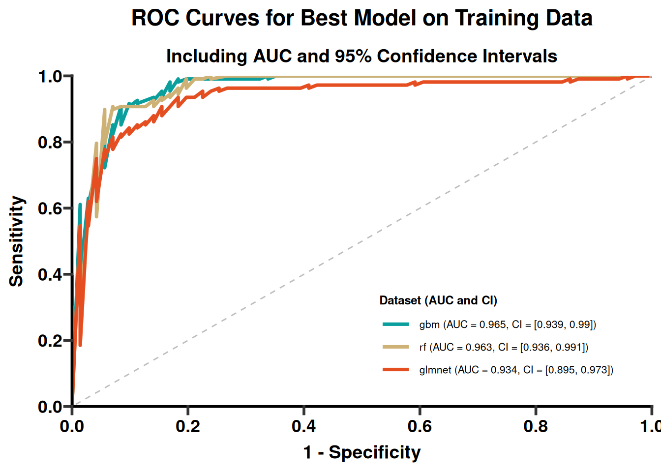
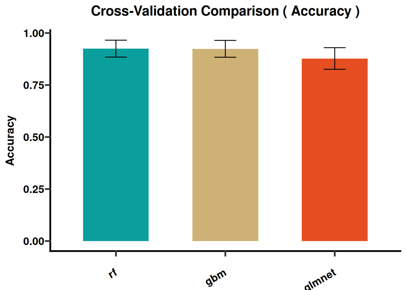
model_obj <- ModelTrainAnalysis(
  object   = model_obj,
  methods  = c("glmnet", "rf", "gbm"),
  save_plots = TRUE,
  seed     = 123,save_dir = "."
)
# ---------------------------------------------------------------------------
````
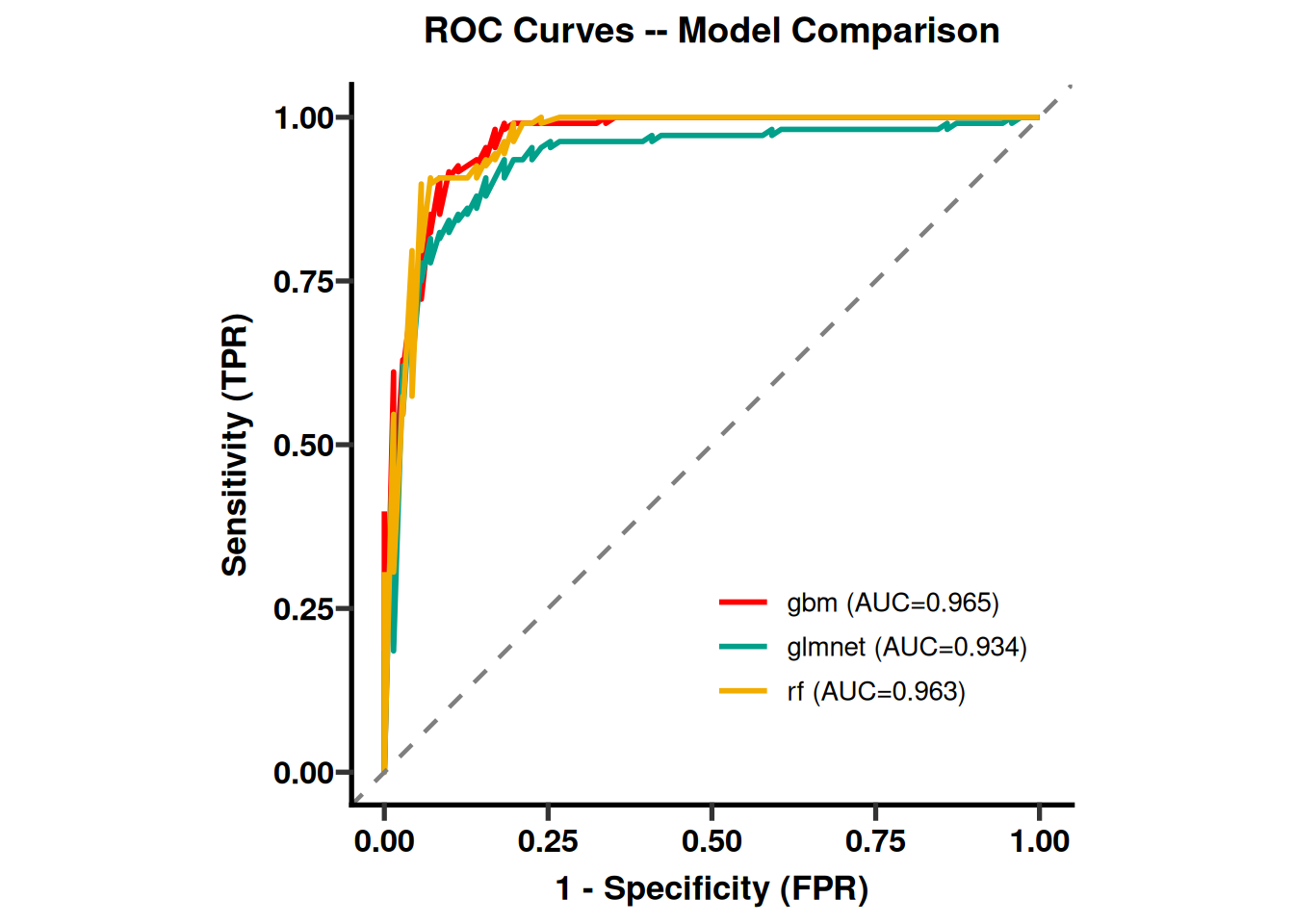
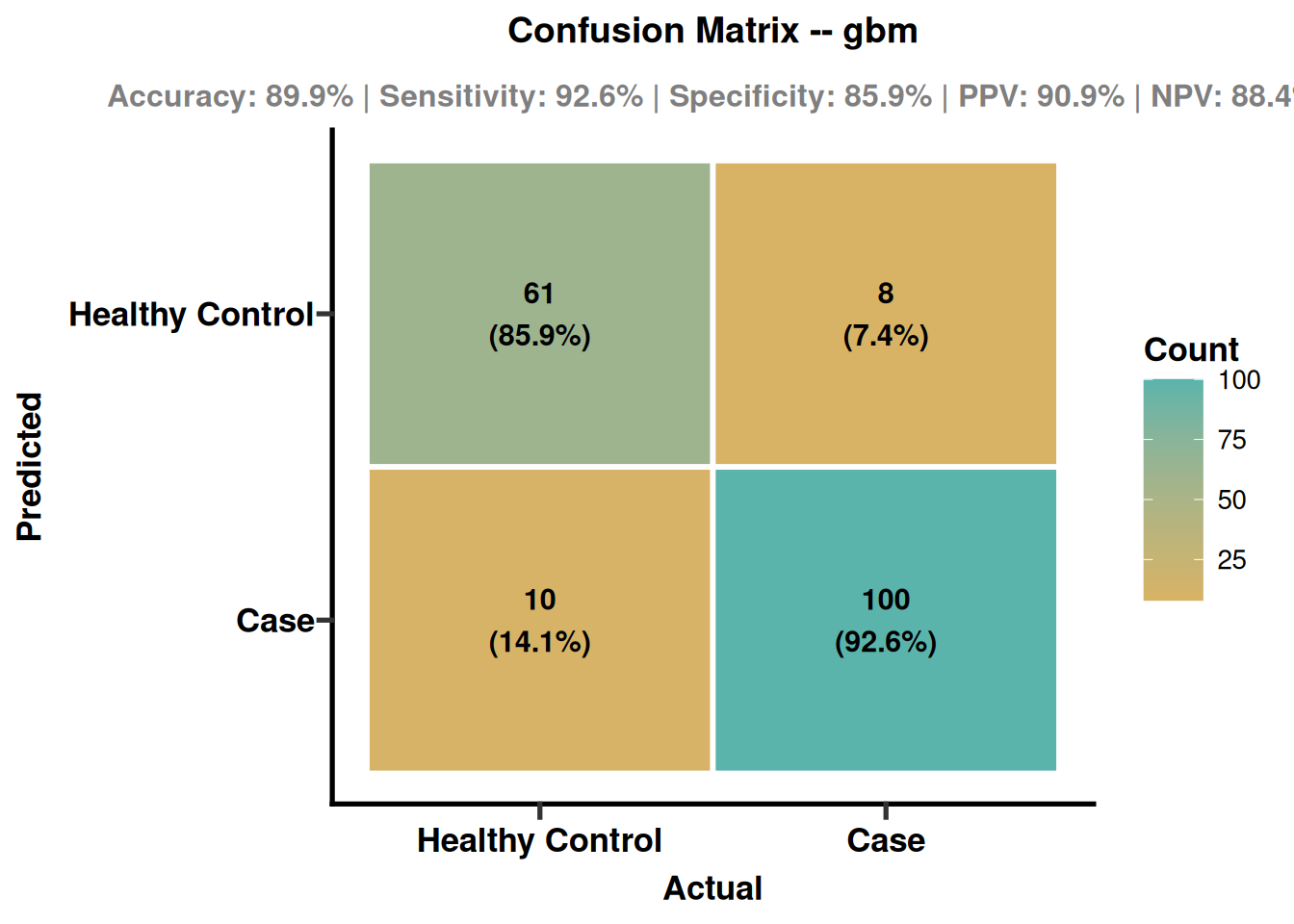
### 5 Pick the best model (by AUC) and look at its performance
This section trains and compares candidate models. Select models using discrimination, calibration, stability, and clinical utility together.
````{r}
#| label: module2-quickstart-06
#| echo: true
#| message: false
#| warning: false
#| fig-show: hold
#| out-width: '100%'
# 5. Pick the best model (by AUC) and look at its performance
# ---------------------------------------------------------------------------
model_obj <- SelectBestModel(model_obj, metric = "auc")
cat("Best model:", model_obj@best.model.result$model_type, "\n")
PlotMultiROC(model_obj, test_data = model_obj@split.scale.data$testing, save_plot = TRUE)
PlotConfusionMatrix(model_obj, test_data = model_obj@split.scale.data$testing,
                    model_name = model_obj@best.model.result$model_type,
                    threshold = 0.5, save_plot = TRUE)
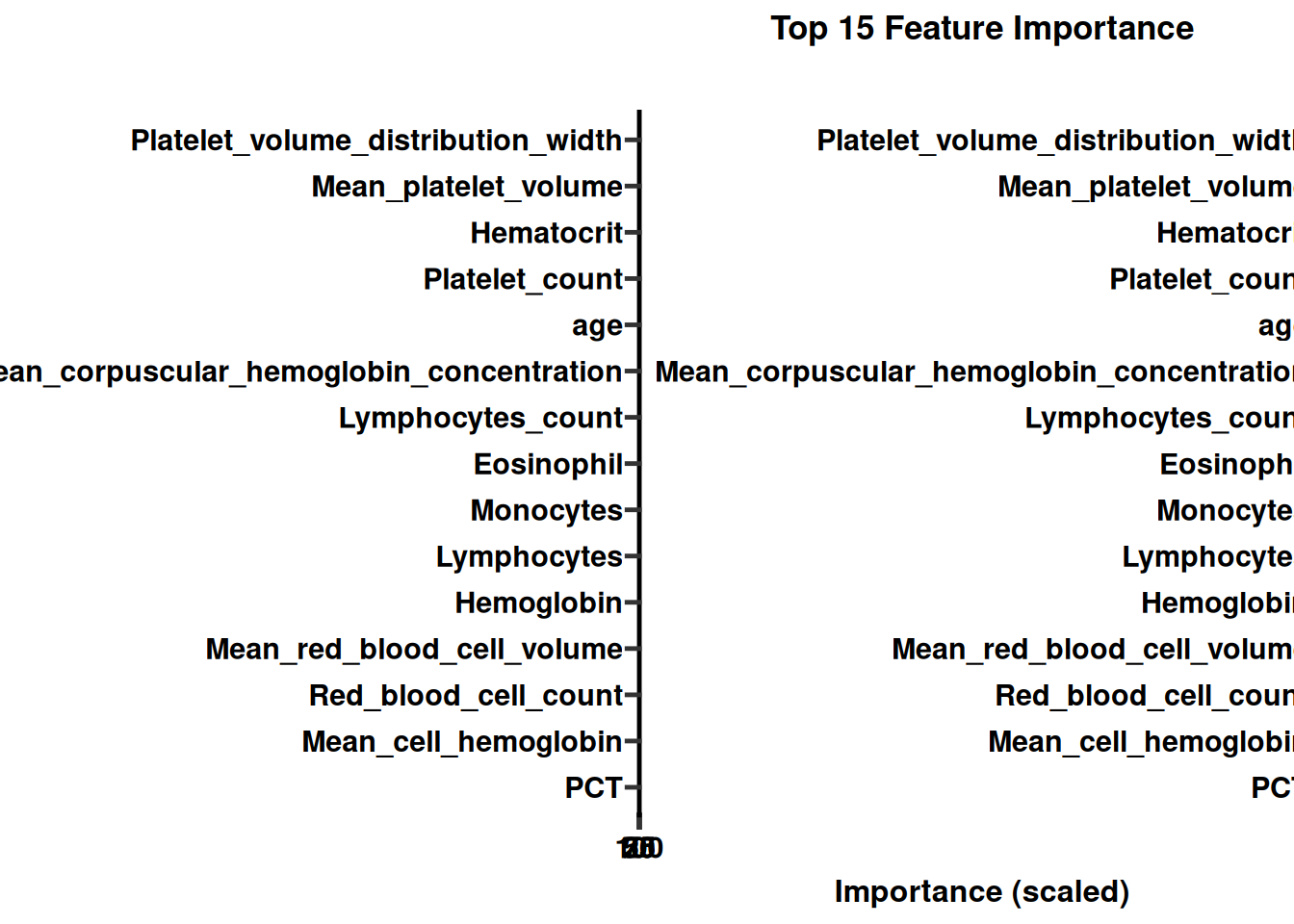
PlotFeatureImportance(model_obj, top_n = 15, save_plot = TRUE)
# ---------------------------------------------------------------------------
````
### 6 Save your trained model
This section trains and compares candidate models. Select models using discrimination, calibration, stability, and clinical utility together.
````{r}
#| label: module2-quickstart-07
#| echo: true
#| message: false
#| warning: false
#| fig-show: hold
#| out-width: '100%'
# 6. Save your trained model
# ---------------------------------------------------------------------------
saveRDS(model_obj, file = "model_obj.rds")

cat("\nDone! model_obj.rds saved.\n",
    "Want ensembles, tuning, SHAP explanations, or clinical thresholds?",
    "See the ADVANCED version of this script.\n")
````