# Module 4: Survival and Prognostic Modeling — Advanced
Using the PMID37633276 example data, the advanced `PrognosiX` workflow keeps development and validation cohorts separate and covers univariable Cox and LASSO-based feature selection, survival-learner benchmarking, tuning, Kaplan–Meier risk groups, subgroup analysis, time-dependent AUC, calibration, nomograms, robustness checks, decision curves, SHAP, and deployment.
## Important Notes
The optional development check runs only when the referenced local package path exists; GitHub and installed-package users can leave it skipped. Main settings are in `OUTPUT_ROOT`, the analysis version, outcome definitions, and the data-import section. Fix the prediction horizons and clinical decision thresholds in the analysis plan before examining validation results.
## Step-by-step Workflow
The workflow is divided into short stages. Each note explains the purpose, key checks, and interpretation limits. Generated plots and tables appear directly below their code chunk.
### About this chapter
**Audience.** Advanced users building and validating a clinical survival model with all diagnostic and explanatory tools.
**Input.** Reads `data/PMID37633276_DIA_plasmaproomic.xlsx` (sheet `Table S1B`) directly.
The chapter runs end to end as one session:
1. **CONFIG & Environment Setup**
2. **Data Preparation (custom Excel data)**
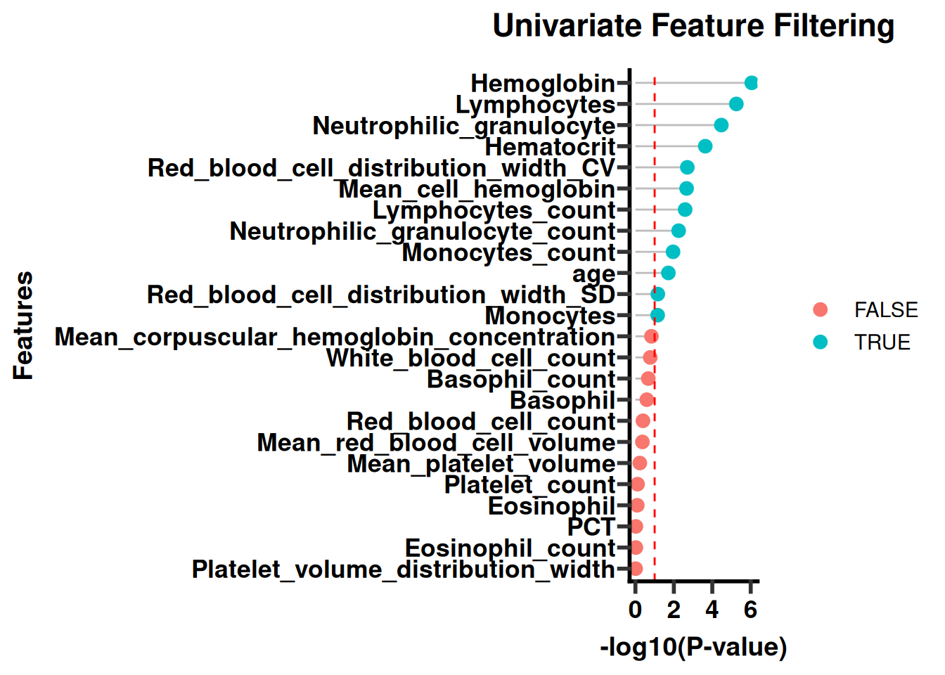
3. **Feature Selection (ONLY on training set)**
4. **Algorithm Benchmarking & Hyperparameter Tuning**
5. **Model Evaluation**
6. **Robustness Analysis**
7. **DCA & SHAP**
8. **Save Final PrognosiX Object**
9. **Deployment: Prediction for New Samples**
10. **Final Report**
### 0 CONFIG & Environment Setup
This section defines seeds, output paths, and dependencies. Update these paths and key parameters first when using new data.
````{r}
#| label: module4-advanced-10
#| cache: false
#| echo: true
#| message: false
#| warning: false
#| fig-show: hold
#| out-width: '100%'
# 0. CONFIG & Environment Setup
# ---------------------------------------------------------------------------
set.seed(2025)

# Define version and output root
VERSION <- "Advanced"
OUTPUT_ROOT <- "./PrognosiX_Output"
OUTPUT_DIR <- file.path(OUTPUT_ROOT, VERSION)

# Load required packages
library(icare)
required_pkgs <- c("mlr3", "mlr3proba", "mlr3viz", "mlr3learners",
                   "survival", "survminer", "ggplot2", "caret", "dplyr",
                   "tidyr", "rms", "risksetROC", "survex", "dcurves",
                   "readxl", "patchwork", "ggrepel", "maxstat")
missing_pkgs <- required_pkgs[!sapply(required_pkgs, requireNamespace, quietly = TRUE)]
if (length(missing_pkgs)) install.packages(missing_pkgs)
invisible(lapply(required_pkgs, library, character.only = TRUE))

# Register OUTPUT_DIR with the package rather than defining a local sub_dir().
# icare already ships sub_dir(); a local definition shadows it only inside this
# script, so functions INSIDE the package that call sub_dir() themselves (e.g.
# plot_tdROC_comparison(), plot_multitime_calibration()) would still resolve it
# in the icare namespace and write to a session-temp directory. Calling
# set_output_root() points both this script and the package at the same tree.
set_output_root(OUTPUT_DIR)

# Create version root and standard subfolders
sub_dir()
sub_dir("data")
sub_dir("01_feature_selection")
sub_dir("02_model")
sub_dir("03_evaluation")
sub_dir("04_robustness")
sub_dir("05_xai")

# ---------------------------------------------------------------------------
````
### 1 Data Preparation (custom Excel data)
This section imports and organizes the data. Check dimensions and variable coding before continuing.
````{r}
#| label: module4-advanced-11
#| cache: false
#| echo: true
#| message: false
#| warning: false
#| fig-show: hold
#| out-width: '100%'
# 1. Data Preparation (custom Excel data)
# ---------------------------------------------------------------------------
raw_dis <- as.data.frame(read_excel("data/PMID37633276_DIA_plasmaproomic.xlsx", sheet = "Table S1B"))
raw_dis <- raw_dis[!grepl(x = raw_dis$`Case ID`, pattern = "^KC"), ]

# Extract numeric features
mat <- raw_dis[, c("White blood cell count",
                   "Lymphocytes%", "Monocytes%", "Neutrophilic granulocyte%", "Eosinophil%",
                   "Basophil%", "Lymphocytes count", "Monocytes count", "Neutrophilic granulocyte count",
                   "Eosinophil count", "Basophil count", "Red blood cell count",
                   "Hemoglobin", "Hematocrit", "Mean red blood cell volume", "Mean cell hemoglobin",
                   "Mean corpuscular hemoglobin concentration", "Red blood cell distribution width CV",
                   "Red blood cell distribution width SD", "Platelet count", "Mean platelet volume",
                   "PCT", "Platelet volume distribution width")]

index <- grepl(x = raw_dis$`Case ID`, pattern = "^HC")

inf <- raw_dis[, c("Case ID", "Sample type", "Plasma proteome ID", "Tissue proteome ID",
                   "Gender", "Age at diagnosis", "Tobacco smoking history", "Drinking history",
                   "Vital status", "Days to last followup", "Days until death",
                   "Combined days to last followup or death", "Progressive-free survival_Status",
                   "Progressive-free survival_Months", "Tumor location", "Tumor size (cm)",
                   "T-category", "Lymph node involvement", "Distant metastasis",
                   "TNM Stage", "Grade", "Morphology")]

# The group label lives in `inf` ONLY -- see the Module 1 chapter for why.
# Keeping it out of the feature matrix also frees its type: readable labels are
# fine, and they become the Table 1 column headers.
inf$group <- factor(ifelse(index, "Healthy Control", "Case"),
                    levels = c("Healthy Control", "Case"))
mat <- as.matrix(mat)
storage.mode(mat) <- "numeric"

rownames(mat) <- inf$`Case ID`
rownames(inf) <- inf$`Case ID`
mat <- as.data.frame(mat)
mat$age <- inf$`Age at diagnosis`
mat$sex <- inf$Gender

inf$time <- inf$`Combined days to last followup or death`
inf$event <- inf$`Vital status`
inf$event <- ifelse(inf$event == "Dead", 1, 0)

# Keep only disease samples (comparing against the label text, not a code --
# the group column is a factor, so `== 1` would silently match nothing)
inf <- inf[inf$group == "Case", ]
mat <- mat[rownames(inf), ]
mat$time <- inf$time
mat$status <- inf$event

stat_obj <- CreateStatObject(
  clean.data = mat,
  info.data = inf,
  group_col = "group",
  na.action = "allow"
)
cat("Stat object created.\n")
prog <- Stat_to_PrognosiX(stat_obj, "time", "status",
                          na_action = "omit",
                          min_events = 10,
                          verbose = TRUE)
# ---------------------------------------------------------------------------
````
### 2 Feature Selection (ONLY on training set)
This section selects candidate features. Consider effect size, stability, and biological plausibility rather than a single significance measure.
````{r}
#| label: module4-advanced-12
#| cache: false
#| echo: true
#| message: false
#| warning: false
#| fig-show: hold
#| out-width: '100%'
# 2. Feature Selection (ONLY on training set)
# ---------------------------------------------------------------------------
task_full <- surv_extract_task(prog)
n <- task_full$nrow
train_idx <- caret::createDataPartition(task_full$data()[[task_full$target_names[2]]],
                                        p = 0.7, list = FALSE)
val_idx <- setdiff(seq_len(n), train_idx)

train_task <- task_full$clone()$filter(train_idx)
val_task <- task_full$clone()$filter(val_idx)

methods_to_run <- c("uni_cox", "lasso", "rf_imp", "ridge", "enet", "vimp")
feat_sel <- surv_feature_selection_multi(
  object = train_task,
  methods = methods_to_run,
  p_threshold = 0.1,
  top_ratio = 0.5,
  combine = "union",
  verbose = TRUE
)
selected_feats <- feat_sel$selected
cat("Selected features:", paste(selected_feats, collapse = ", "), "\n")
write.csv(feat_sel$method_table,
          file = file.path(sub_dir("01_feature_selection"), "feature_selection_methods.csv"),
          row.names = FALSE)

train_task <- train_task$select(selected_feats)
val_task <- val_task$select(selected_feats)

# Save train/validation data
train_data <- as.data.frame(train_task$data())
val_data <- as.data.frame(val_task$data())
write.csv(train_data, file = file.path(sub_dir("data"), "training_data.csv"), row.names = FALSE)
write.csv(val_data,   file = file.path(sub_dir("data"), "validation_data.csv"), row.names = FALSE)

# ---------------------------------------------------------------------------
````
### 3 Algorithm Benchmarking & Hyperparameter Tuning
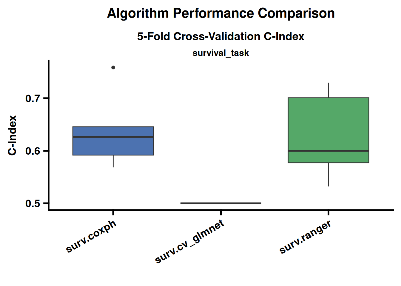
This section trains and compares candidate models. Select models using discrimination, calibration, stability, and clinical utility together.
````{r}
#| label: module4-advanced-13
#| cache: false
#| echo: true
#| message: false
#| warning: false
#| fig-show: hold
#| out-width: '100%'
# 3. Algorithm Benchmarking & Hyperparameter Tuning
# ---------------------------------------------------------------------------
learners_list <- list(
  surv_get_learner("surv.coxph",     train_task),
  surv_get_learner("surv.cv_glmnet", train_task),
  surv_get_learner("surv.ranger",    train_task)
)
bmr1 <- surv_run_algorithm_benchmark(train_task, learners_list)
dev.new()
bmr2 <- surv_benchmark_learners(train_task, learner_ids = c("surv.coxph", "surv.ranger"), tune = FALSE)
bmr2_summary <- surv_summarize_benchmark(bmr2)
write.csv(bmr2_summary, file = file.path(sub_dir("02_model"), "algorithm_benchmark.csv"), row.names = FALSE)

best_id <- "surv.ranger"
tune <- surv_train_and_tune(train_task, best_id, tuning_budget = 25)
best_lrn <- tune$learner
cv_cindex <- tune$cv_performance
cat("CV C-index after tuning:", round(cv_cindex, 4), "\n")
# ---------------------------------------------------------------------------
````
### 4 Model Evaluation
This section trains and compares candidate models. Select models using discrimination, calibration, stability, and clinical utility together.
````{r}
#| label: module4-advanced-14
#| cache: false
#| echo: true
#| message: false
#| warning: false
#| fig-show: hold
#| out-width: '100%'
# 4. Model Evaluation
# ---------------------------------------------------------------------------
best_lrn$predict_type <- "distr"
train_perf <- surv_evaluate_model(best_lrn, train_task,
                                  measures = list(msr("surv.cindex"), msr("surv.graf")))
cat("Training apparent C-index:", round(train_perf$surv.cindex, 4), "\n")
val_pred <- best_lrn$predict(val_task)
val_cindex <- val_pred$score(msr("surv.cindex"))
cat("Validation C-index:", round(val_cindex, 4), "\n")
# Save performance metrics
perf_df <- data.frame(
  Dataset = c("Training", "Validation"),
  C_index = c(train_perf$surv.cindex, val_cindex)
)
write.csv(perf_df, file = file.path(sub_dir("03_evaluation"), "performance.csv"), row.names = FALSE)

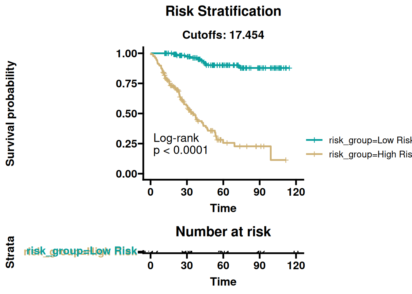
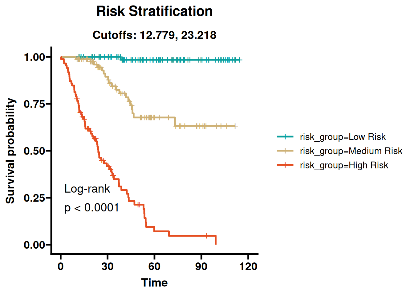
# ---- 4.1 KM Curves ----
# IMPORTANT: The following KM curves and the cutoff derived from the training set
# are APPARENT (optimistic) performance. They are useful for internal exploration
# but MUST be re‑evaluated on an independent validation set before reporting.
pred_train <- best_lrn$predict(train_task)
cut_df <- as.data.frame(train_task$data())
cut_df$risk <- pred_train$crank

# Compute optimal cutoff using multiple methods.
# For publication, consider using 'maxstat' (Hothorn & Lausen, 2003) with
# bootstrap resampling to obtain a stable, data‑driven threshold.
# The 'p_optimize' method is also provided for historical consistency.
cut_res <- tryCatch({
  surv_cutpoint(cut_df, time = "time", event = "status", variables = "risk")
}, error = function(e) {
  warning("surv_cutpoint failed: ", e$message, ". Using median split.")
  list(cutpoint = data.frame(cutpoint = median(cut_df$risk, na.rm = TRUE)))
})
opt_cutoff <- cut_res$cutpoint$cutpoint
cat("Optimal cutoff (from surv_cutpoint):", round(opt_cutoff, 4), "\n")
# Generate KM plots for different cutoff methods
# Note: 'p_optimize' and 'maxstat' use bootstrap/maximally selected statistics
# and are exploratory; their p‑values should not be used as confirmatory.
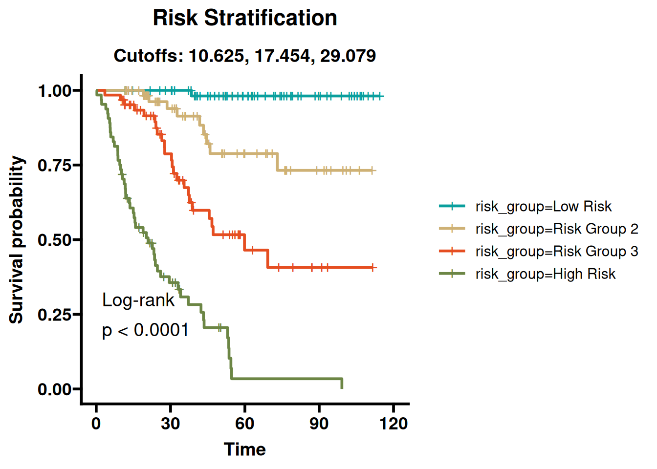
km_median    <- surv_plot_risk_km(best_lrn, train_task, "median", risk_table = TRUE)
km_tertile   <- surv_plot_risk_km(best_lrn, train_task, "tertile")
km_quartile  <- surv_plot_risk_km(best_lrn, train_task, "quartile")
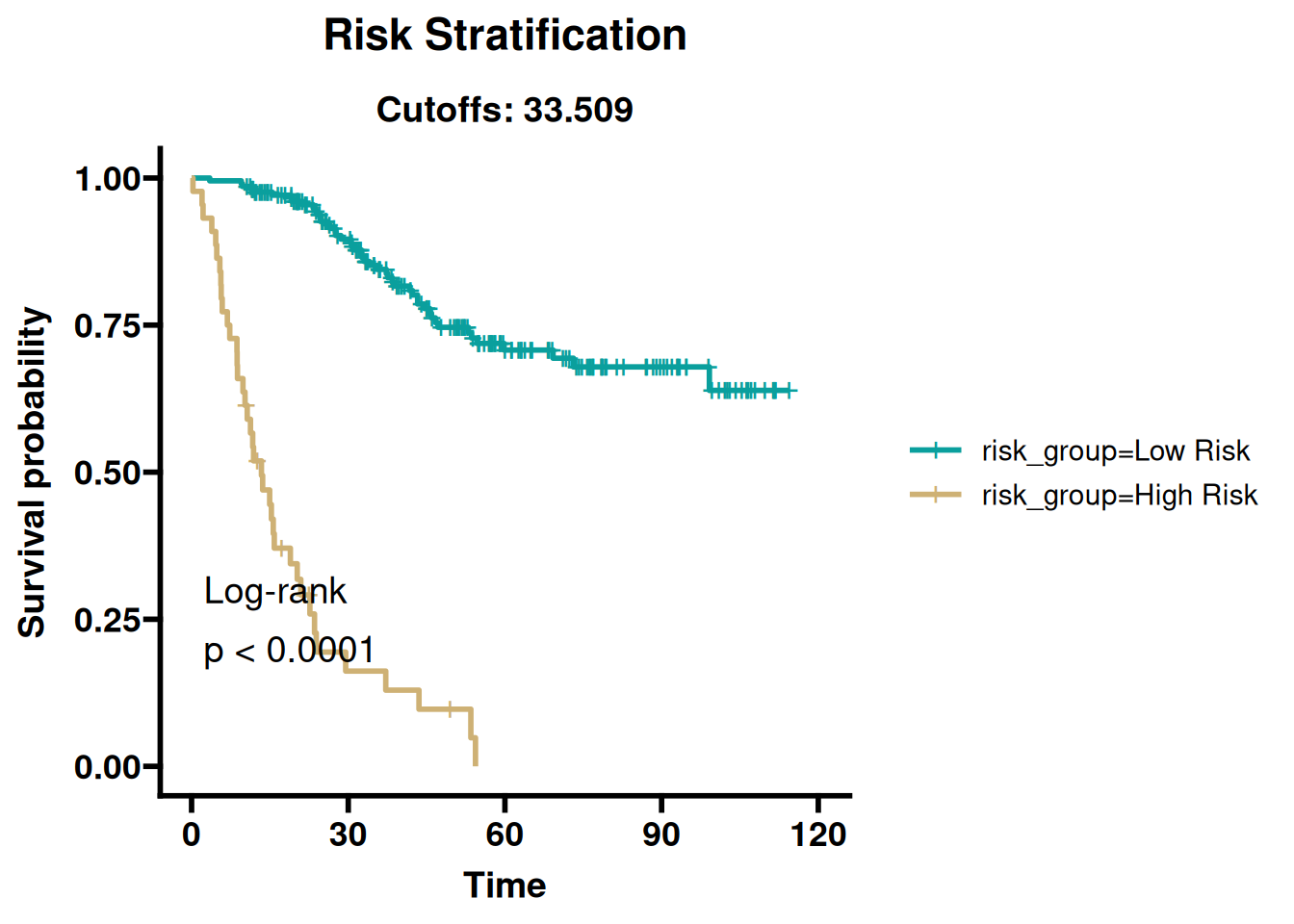
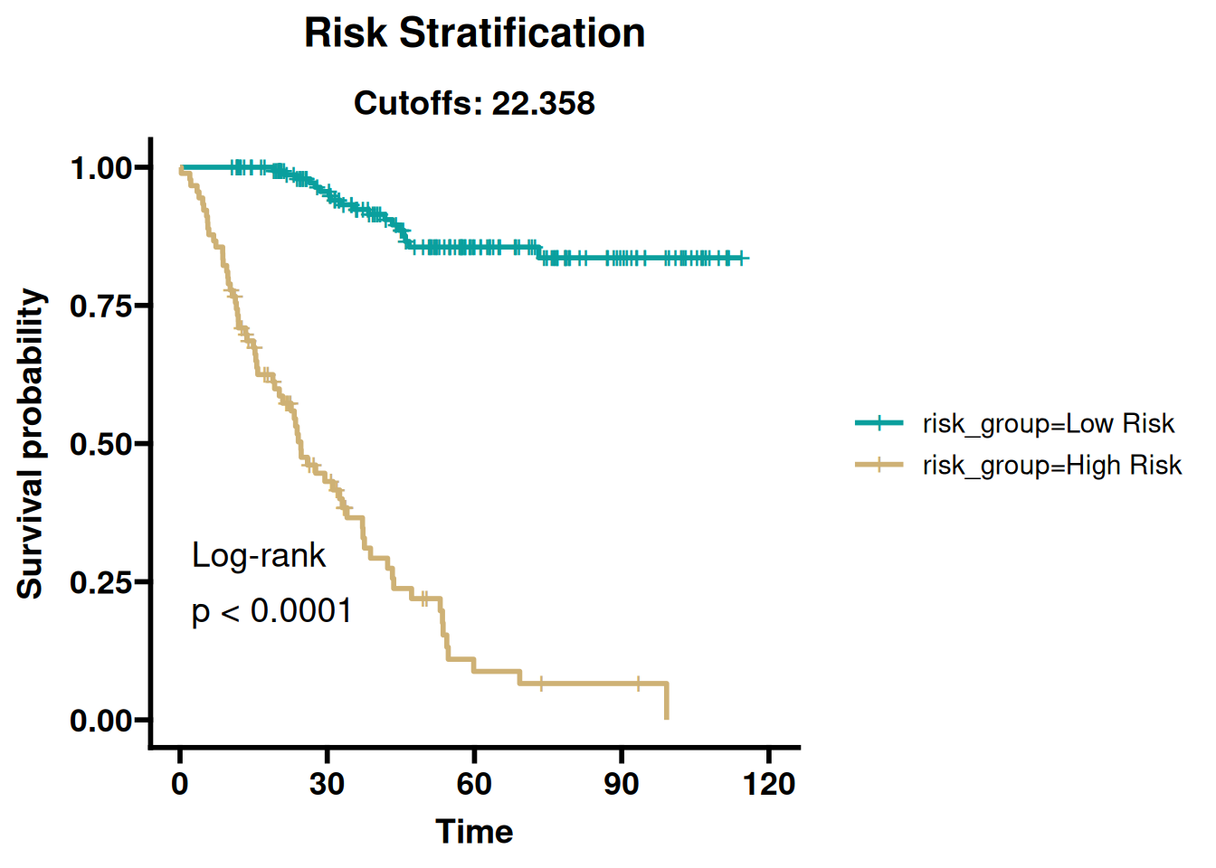
km_p_optimize <- surv_plot_risk_km(best_lrn, train_task, "p_optimize",
                                   n_boot = 100, fraction = 0.7)
km_maxstat   <- surv_plot_risk_km(best_lrn, train_task, "maxstat",
                                  n_boot = 100, minprop = 0.3)

# Save training KM plots
print(km_median)

print(km_tertile)

print(km_quartile)

print(km_p_optimize)

print(km_maxstat)

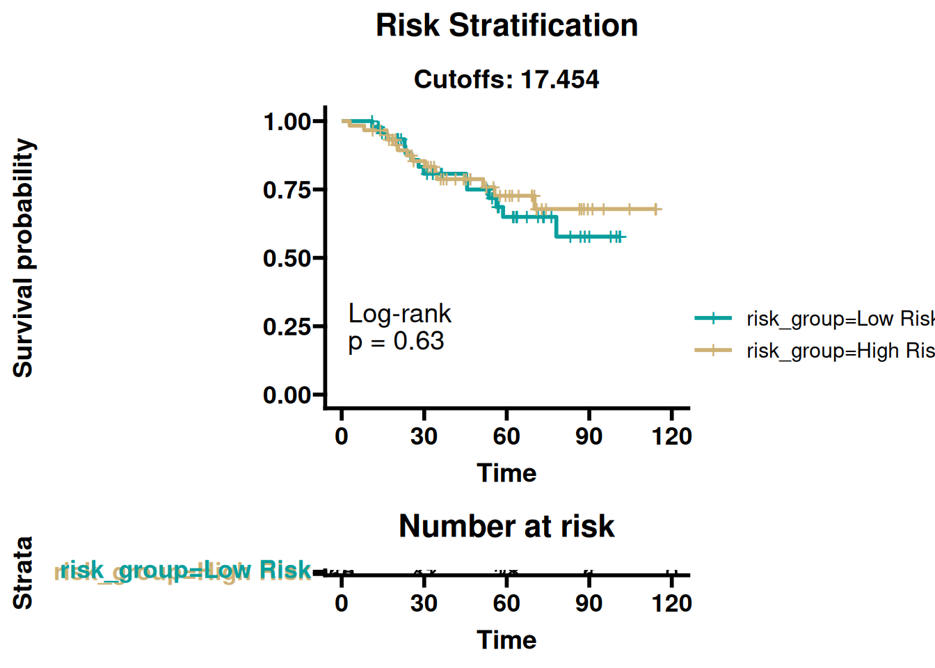
# Apply a fixed cutoff (here we use the median from training) to the validation set
train_cutoff <- get_cf(km_median)
if (is.null(train_cutoff)) train_cutoff <- opt_cutoff
km_val_fixed <- surv_plot_risk_km(best_lrn, val_task,
                                  cutoff_method = "custom",
                                  custom_cutoffs = train_cutoff,
                                  risk_table = TRUE)

print(km_val_fixed)

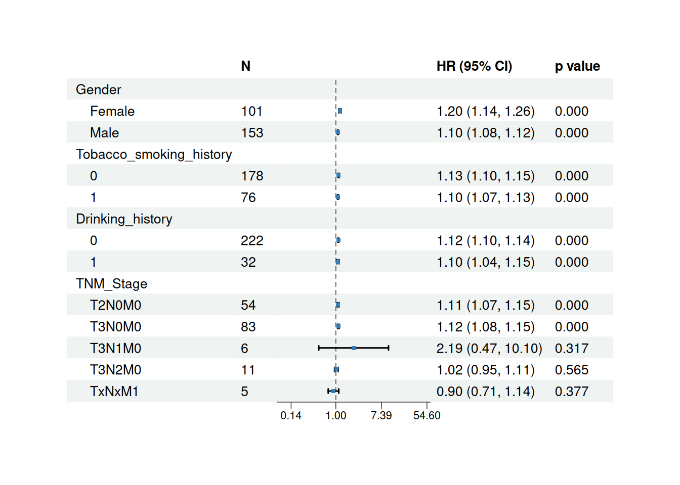
# ---- 4.2 Subgroup Forest (FIXED: use subsetted prog) ----
# Subset prog to training samples to match train_task rows
train_prog <- prog
train_prog@clean.data <- prog@clean.data[train_idx, , drop = FALSE]
train_prog@info.data <- prog@info.data[train_idx, , drop = FALSE]
train_prog@survival.data <- prog@survival.data[train_idx, , drop = FALSE]

clinical_cols <- colnames(train_prog@info.data)
# info.data names are normalised by CreateStatObject(): spaces and dots become
# underscores. Passing the dotted spelling would make intersect() drop
# everything except "Gender" and silently shrink the subgroup forest.
candidate_vars <- c("Gender", "Tobacco_smoking_history", "Drinking_history", "TNM_Stage")
subgroup_vars <- intersect(candidate_vars, clinical_cols)

forest <- surv_plot_subgroup_forest(
  learner = best_lrn,
  object = train_task,
  subgroup_vars = subgroup_vars,
  prog = train_prog,
  save_plot = TRUE,
  save_dir = sub_dir("03_evaluation"),
  file_name = "subgroup_forest.pdf"
)
print(forest)
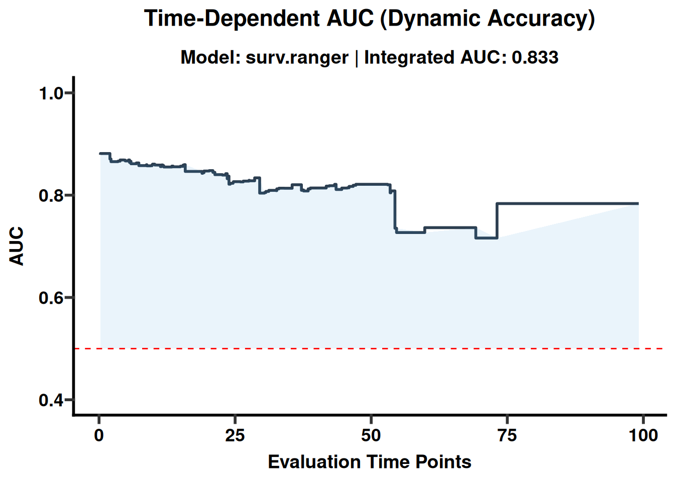
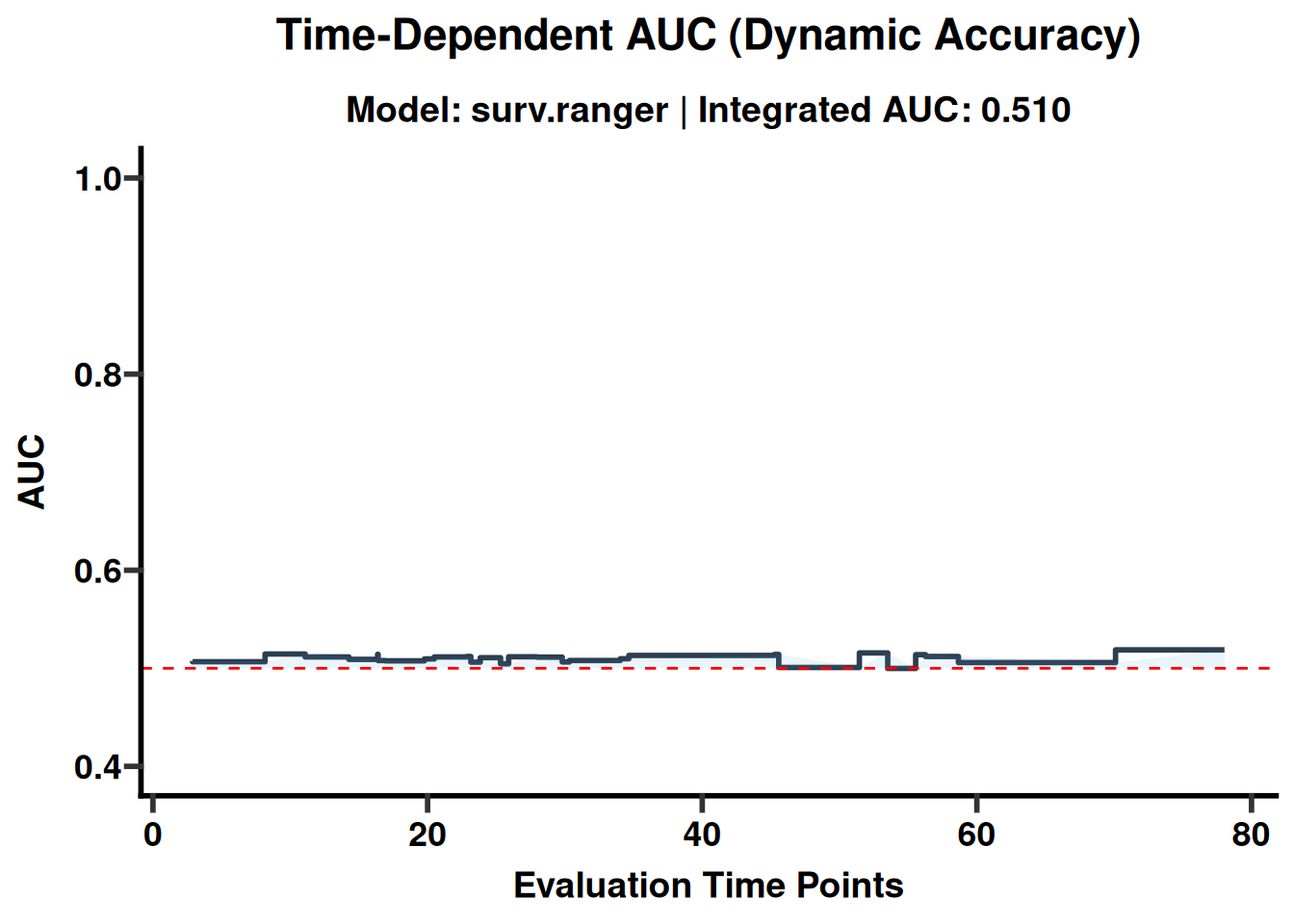
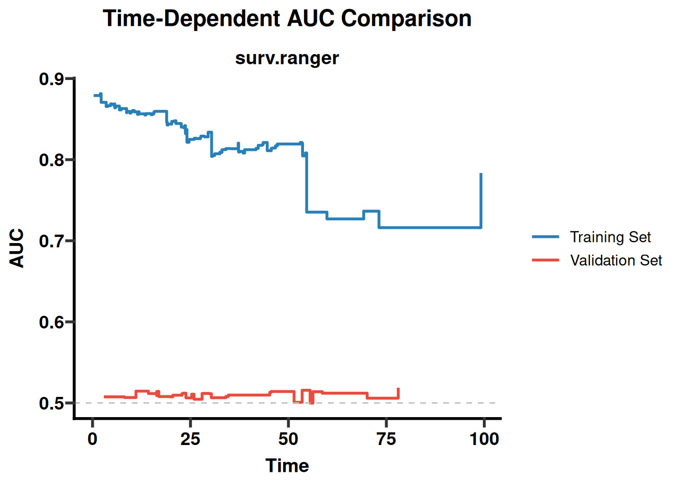
# ---- 4.3 Time-dependent AUC ----
# Note: These are also apparent performance when computed on the training set.
auc_train <- surv_plot_time_dependent_auc(best_lrn, train_task)
auc_val   <- surv_plot_time_dependent_auc(best_lrn, val_task)
auc_cmp   <- surv_plot_comparison_auc(best_lrn, train_task, val_task)
ggsave(file.path(sub_dir("03_evaluation"), "AUC_comparison.pdf"), auc_cmp, width = 8, height = 5)

# ---- 4.4 Calibration ----
cal_train <- surv_plot_calibration(best_lrn, train_task, time_point = 200)
cal_cmp <- surv_plot_comparison_calibration(best_lrn, train_task, val_task, time_point = 200)
ggsave(file.path(sub_dir("03_evaluation"), "Calibration_train.pdf"), cal_train, width = 8, height = 6)
ggsave(file.path(sub_dir("03_evaluation"), "Calibration_comparison.pdf"), cal_cmp, width = 8, height = 6)

# ---- 4.5 External Validation (using validation set) ----
val_data_ext <- as.data.frame(task_full$data())[val_idx, selected_feats, drop = FALSE]
val_data_ext$time <- task_full$data()[[task_full$target_names[1]]][val_idx]
val_data_ext$status <- task_full$data()[[task_full$target_names[2]]][val_idx]
val_res <- surv_predict_on_validation(best_lrn, val_data_ext, train_task)
val_cindex_alt <- val_res$prediction$score(msr("surv.cindex"))
cat("Validation C-index (alt):", round(val_cindex_alt, 4), "\n")
# ---- 4.6 Nomogram ----
# The revized surv_generate_nomogram now includes a proportional hazards test
# (cox.zph) which will be printed to the console. If any variable violates
# the PH assumption, a warning is shown.
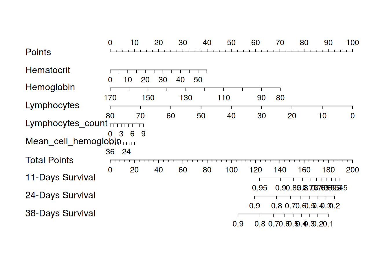
nom <- surv_generate_nomogram(train_task,
                              selected_features = head(selected_feats, 5),
                              time_points = c(90, 180, 365),
                              time_unit = "days")
# Nomogram is drawn; optionally save via pdf().

# ---------------------------------------------------------------------------
````
### 5 Robustness Analysis
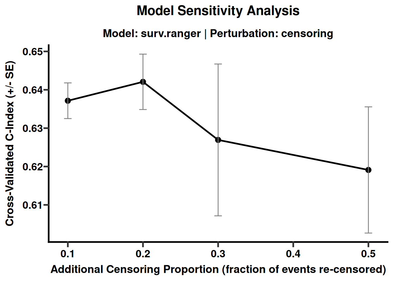
This section tests sensitivity to sampling, censoring, and feature changes. Robust conclusions should remain similar under reasonable perturbations.
````{r}
#| label: module4-advanced-15
#| cache: false
#| echo: true
#| message: false
#| warning: false
#| fig-show: hold
#| out-width: '100%'
# 5. Robustness Analysis
# ---------------------------------------------------------------------------
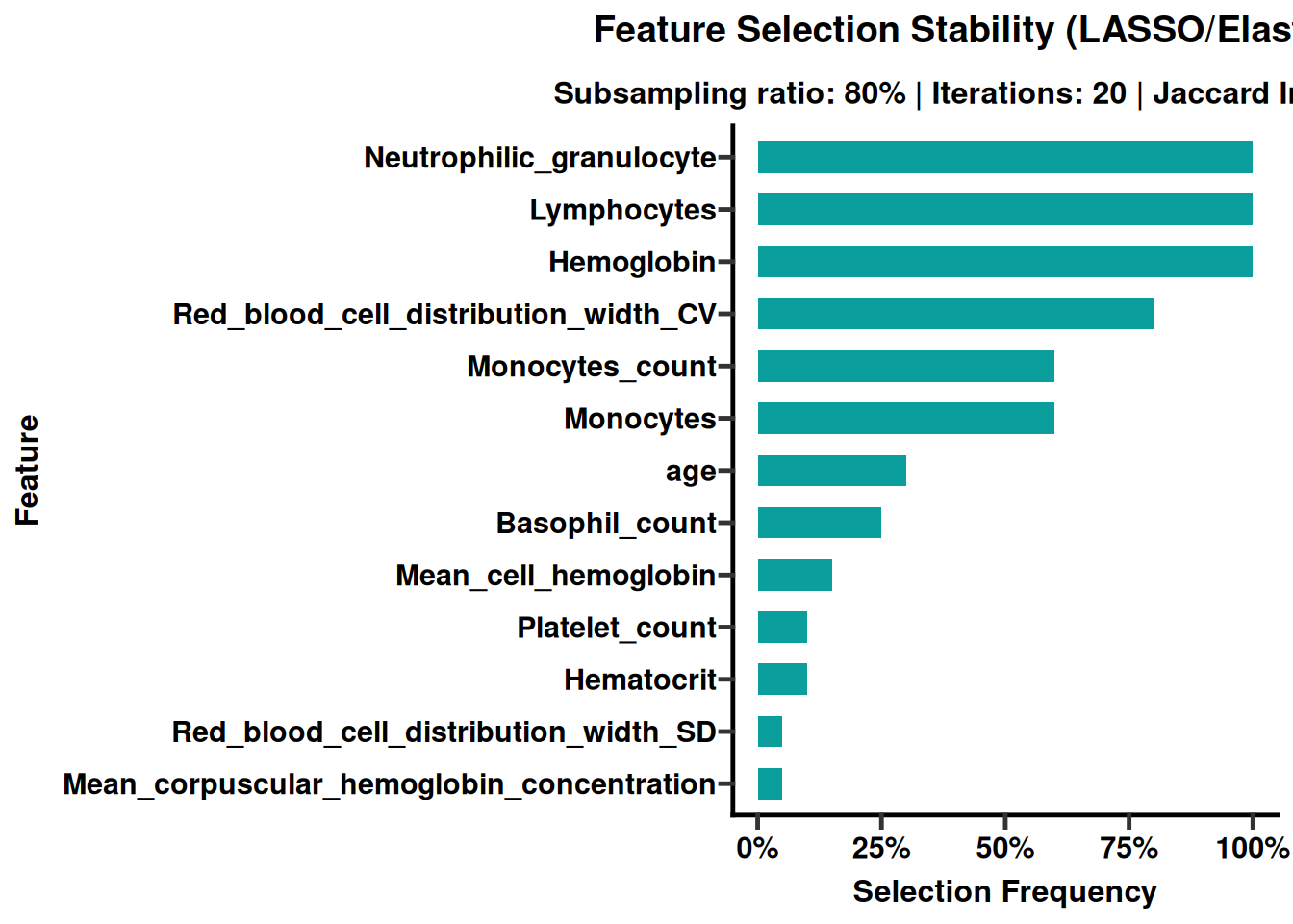
stab <- surv_analyze_feature_stability(train_task, "time", "status", n_repeat = 20, alpha = 1)
cat("Stability index:", round(stab$stability_index, 4), "\n")
ggsave(file.path(sub_dir("04_robustness"), "stability_plot.pdf"), stab$plot, width = 8, height = 6)
write.csv(stab$frequencies, file.path(sub_dir("04_robustness"), "stability_frequencies.csv"), row.names = FALSE)

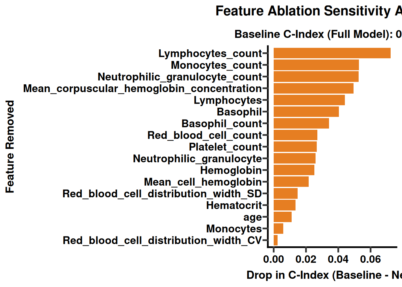
abl <- surv_analyze_feature_ablation(train_task, best_id, selected_feats)
ggsave(file.path(sub_dir("04_robustness"), "ablation_plot.pdf"), abl$plot, width = 8, height = 6)
write.csv(abl$results, file.path(sub_dir("04_robustness"), "ablation_results.csv"), row.names = FALSE)

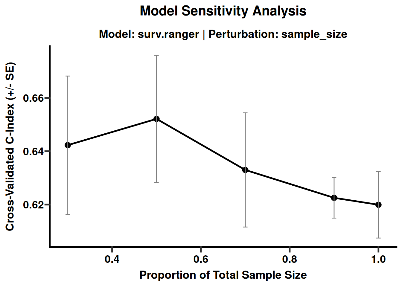
sens_sample <- surv_analyze_model_sensitivity(train_task, best_id, analysis_type = "sample_size")
sens_censor <- surv_analyze_model_sensitivity(train_task, best_id, analysis_type = "censoring")
ggsave(file.path(sub_dir("04_robustness"), "sensitivity_sample.pdf"), sens_sample$plot, width = 8, height = 5)
ggsave(file.path(sub_dir("04_robustness"), "sensitivity_censor.pdf"), sens_censor$plot, width = 8, height = 5)
write.csv(sens_sample$results, file.path(sub_dir("04_robustness"), "sensitivity_sample.csv"), row.names = FALSE)
write.csv(sens_censor$results, file.path(sub_dir("04_robustness"), "sensitivity_censor.csv"), row.names = FALSE)

# ---------------------------------------------------------------------------
````
### 6 DCA & SHAP
This section examines clinical utility and model explanations. Explanatory plots describe model behavior and do not establish causality.
````{r}
#| label: module4-advanced-16
#| cache: false
#| echo: true
#| message: false
#| warning: false
#| fig-show: hold
#| out-width: '100%'
# 6. DCA & SHAP
# ---------------------------------------------------------------------------
val_time <- val_task$data()[[val_task$target_names[1]]]
val_status <- val_task$data()[[val_task$target_names[2]]]
event_times <- val_time[val_status == 1]
if (length(event_times) == 0) stop("No events in validation set.")
eval_time <- round(quantile(event_times, 0.5, na.rm = TRUE), 0)
if (eval_time < min(event_times)) eval_time <- min(event_times)
cat("Using eval_time =", eval_time, "for DCA\n")
dca_res <- plot_dca_survival(
  learners = list("Tuned" = best_lrn),
  object = val_task,
  eval_time = eval_time,
  clin_range = c(0.05, 0.5),
  print_stats = TRUE
)
ggsave(file.path(sub_dir("05_xai"), "dca_plot.pdf"), dca_res$plot, width = 7, height = 5)
write.csv(dca_res$table, file.path(sub_dir("05_xai"), "dca_table.csv"), row.names = FALSE)

shap_global <- surv_explain_shap(
  learner = best_lrn,
  task = val_task,
  type = "global",
  n_explain = 30,
  n_background = 10,
  n_timepoints = 10,
  n_top_features = 6,
  verbose = TRUE
)
ggsave(file.path(sub_dir("05_xai"), "shap_global_bar.pdf"), shap_global$plots$bar_plot, width = 8, height = 6)
if (!is.null(shap_global$plots$line_plot)) {
  ggsave(file.path(sub_dir("05_xai"), "shap_global_line.pdf"), shap_global$plots$line_plot, width = 8, height = 6)
}
write.csv(shap_global$shap_long, file.path(sub_dir("05_xai"), "shap_values_global.csv"), row.names = FALSE)

beeswarm_plot <- surv_plot_shap_beeswarm(shap_global, top_n = 6, method = "beeswarm",
                                         title = "Global SurvSHAP (validation set)")
ggsave(file.path(sub_dir("05_xai"), "shap_beeswarm.pdf"), beeswarm_plot, width = 9, height = 6)

# ---------------------------------------------------------------------------
````
### 7 Save Final PrognosiX Object
This section saves model objects, tables, and figures for reproducibility, review, and reuse.
````{r}
#| label: module4-advanced-17
#| cache: false
#| echo: true
#| message: false
#| warning: false
#| fig-show: hold
#| out-width: '100%'
# 7. Save Final PrognosiX Object
# ---------------------------------------------------------------------------
prog@best.model <- list(
  learner_id = best_id,
  learner = best_lrn,
  best_params = tune$best_params,
  cv_cindex = cv_cindex,
  features = selected_feats,
  cutoff = opt_cutoff,
  decision_type = "binary",
  train_cols = train_task$feature_names
)
prog@subgroup.risk <- list(
  benchmark_table = bmr1$table,
  stability = stab,
  ablation = abl,
  validation = list(cindex = val_cindex, n = val_task$nrow)
)
prog@split.data <- list(train_idx = train_idx, val_idx = val_idx)
saveRDS(prog, file = file.path(sub_dir("data"), "prog_obj_final.rds"))

# ---------------------------------------------------------------------------
````
### 8 Deployment: Prediction for New Samples
This section applies the trained object to new samples. Validate input format, performance, and target population in an independent cohort before deployment.
````{r}
#| label: module4-advanced-19
#| cache: false
#| echo: true
#| message: false
#| warning: false
#| fig-show: hold
#| out-width: '100%'
# 8. Deployment: Prediction for New Samples
# ---------------------------------------------------------------------------
# Instead of the veteran example, use actual rows from your training data
# (or real new data) that contain all selected features.
# For demonstration, we take the first 2 rows of the original feature matrix.
#new_patients <- data.frame(
#  Mean_corpuscular_hemoglobin_concentration = c(33, 34),
#  Basophil_count = c(0.02, 0.03),
#  Monocytes = c(0.6, 0.7),
#  Neutrophilic_granulocyte = c(4.2, 5.1),
#  Red_blood_cell_distribution_width_CV = c(12.3, 11.8),
#  Mean_red_blood_cell_volume = c(89, 92),
#  Lymphocytes_count = c(1.8, 2.1),
#  Platelet_volume_distribution_width = c(12.0, 13.1),
#  Lymphocytes = c(1.8, 2.1),   # note: this may be same as Lymphocytes_count? check your data
#  Monocytes_count = c(0.6, 0.7),
#  Neutrophilic_granulocyte_count = c(4.2, 5.1),
#  Mean_platelet_volume = c(10.5, 11.0),
#  row.names = c("patient_1", "patient_2")
#)

#risk_scores <- predict_prognosix(prog, new_patients, impute = TRUE)
#pred_groups_med <- predict_risk_groups(prog, new_patients, cutoff_method = "median")
#pred_groups_cus <- predict_risk_groups(prog, new_patients,
#                                       cutoff_method = "custom",
#                                       custom_cutoffs = opt_cutoff)
#cat("Risk scores:\n"); print(risk_scores)
#cat("Median groups:\n"); print(pred_groups_med)
#cat("Custom groups:\n"); print(pred_groups_cus)

manager <- New_Prog_Manager(prog)
if (interactive()) {
  use_app_theme_grey()
  set_prog_app_text(
    title = "Survival Risk Predictor",
    citation_text = "Data: PMID37633276_DIA_plasmaproomic cohort."
  )
  set_prog_app_theme(
    primary_color = "#2c7fb8", background_color = "#f0f4f8", sidebar_color = "#e9ecef",
    box_background = "#ffffff", label_color = "#2c7fb8",
    run_button_gradient_start = "#2c7fb8", run_button_gradient_end = "#1d4e6e",
    risk_high_color = "#d9534f", risk_medium_color = "#f0ad4e", risk_low_color = "#5cb85c",
    table_header_color = "#2c7fb8", font_family = "Arial, sans-serif", font_size_base = 14
  )
  launch_prog_deploy_app(
    manager,
    var_dict = data.frame(
      Feature = selected_feats,
      Description = paste("Predictor", seq_along(selected_feats)),
      Units = rep("--", length(selected_feats))
    ),
    project_info = list(
      abstract = paste("Prognostic model trained on", train_task$nrow, "patients."),
      citation = "PMID37633276_DIA_plasmaproomic cohort."
    )
  )
}

# ---------------------------------------------------------------------------
````
### 9 Final Report
This section saves model objects, tables, and figures for reproducibility, review, and reuse.
````{r}
#| label: module4-advanced-20
#| cache: false
#| echo: true
#| message: false
#| warning: false
#| fig-show: hold
#| out-width: '100%'
# 9. Final Report
# ---------------------------------------------------------------------------
cat("\n========================================\n")
cat("Module 4 (advanced, leakage‑free) finished successfully!\n")
cat("Best model:", best_id,
    "| CV C-index (training):", round(cv_cindex, 4),
    "| Validation C-index:", round(val_cindex, 4), "\n")
cat("Optimal cutoff:", round(opt_cutoff, 4), "\n")
cat("All results saved under:", OUTPUT_DIR, "\n")
cat("========================================\n")
````