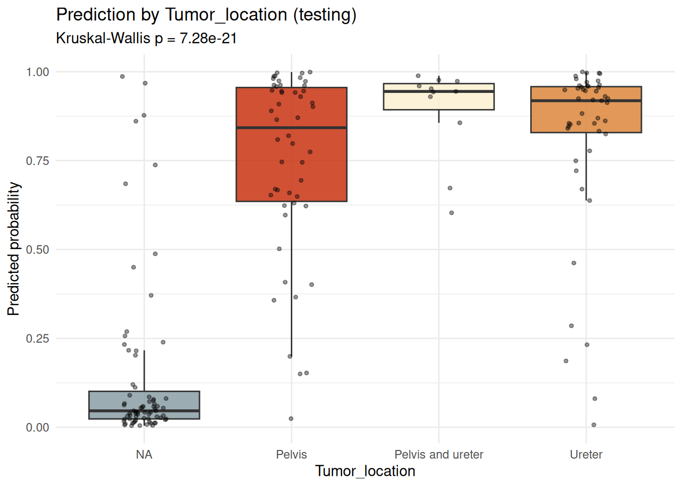
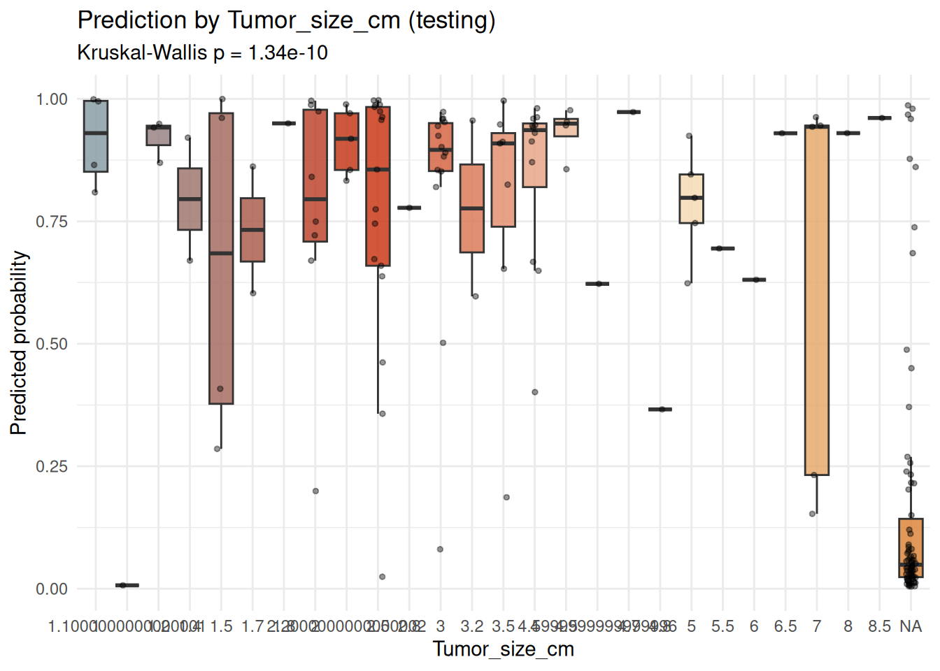
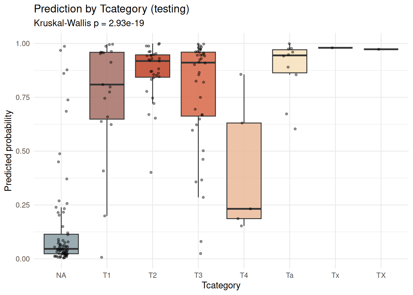
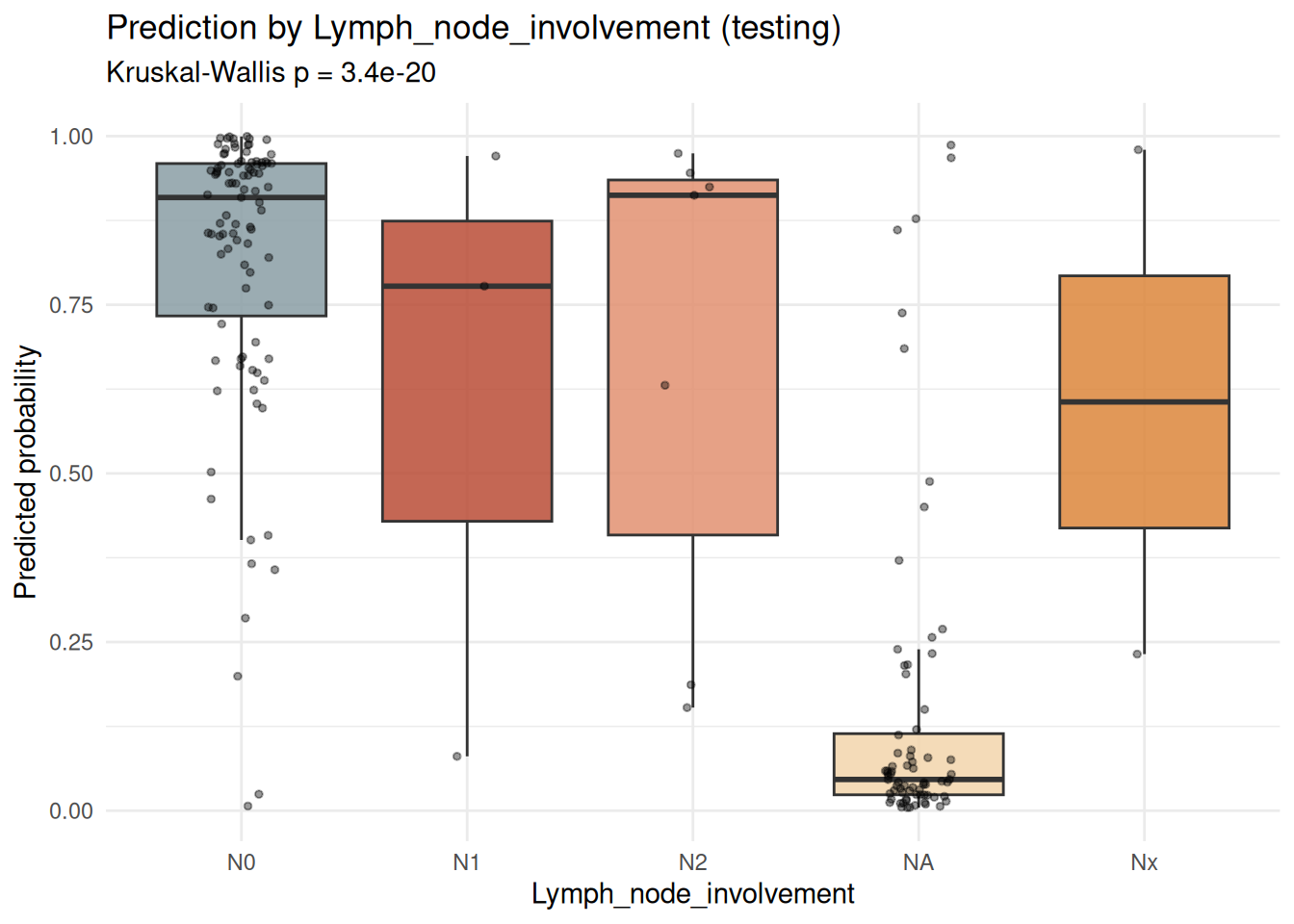
# Module 2: Classification Modeling — Advanced
The advanced `Train_Model` workflow covers algorithm availability checks, RFE/GA/SA and built-in feature selection, preprocessing benchmarks, model comparison, ensembles, hyperparameter tuning, SHAP and DALEX explanations, clinically interpretable thresholds, NRI/IDI, deployment, and an optional Shiny interface.
## Key Configuration
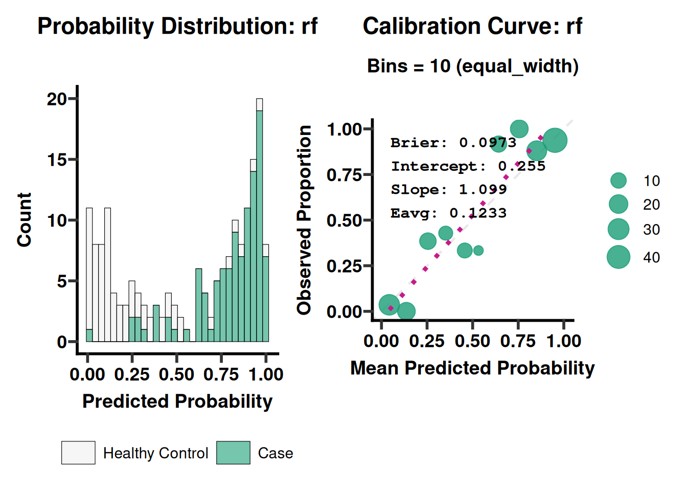
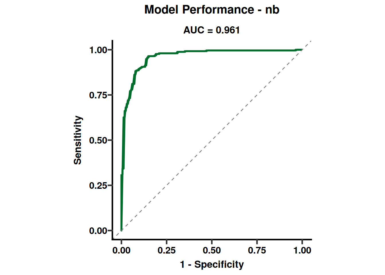
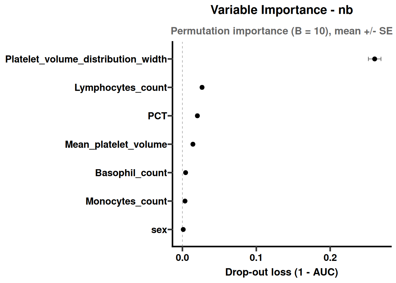
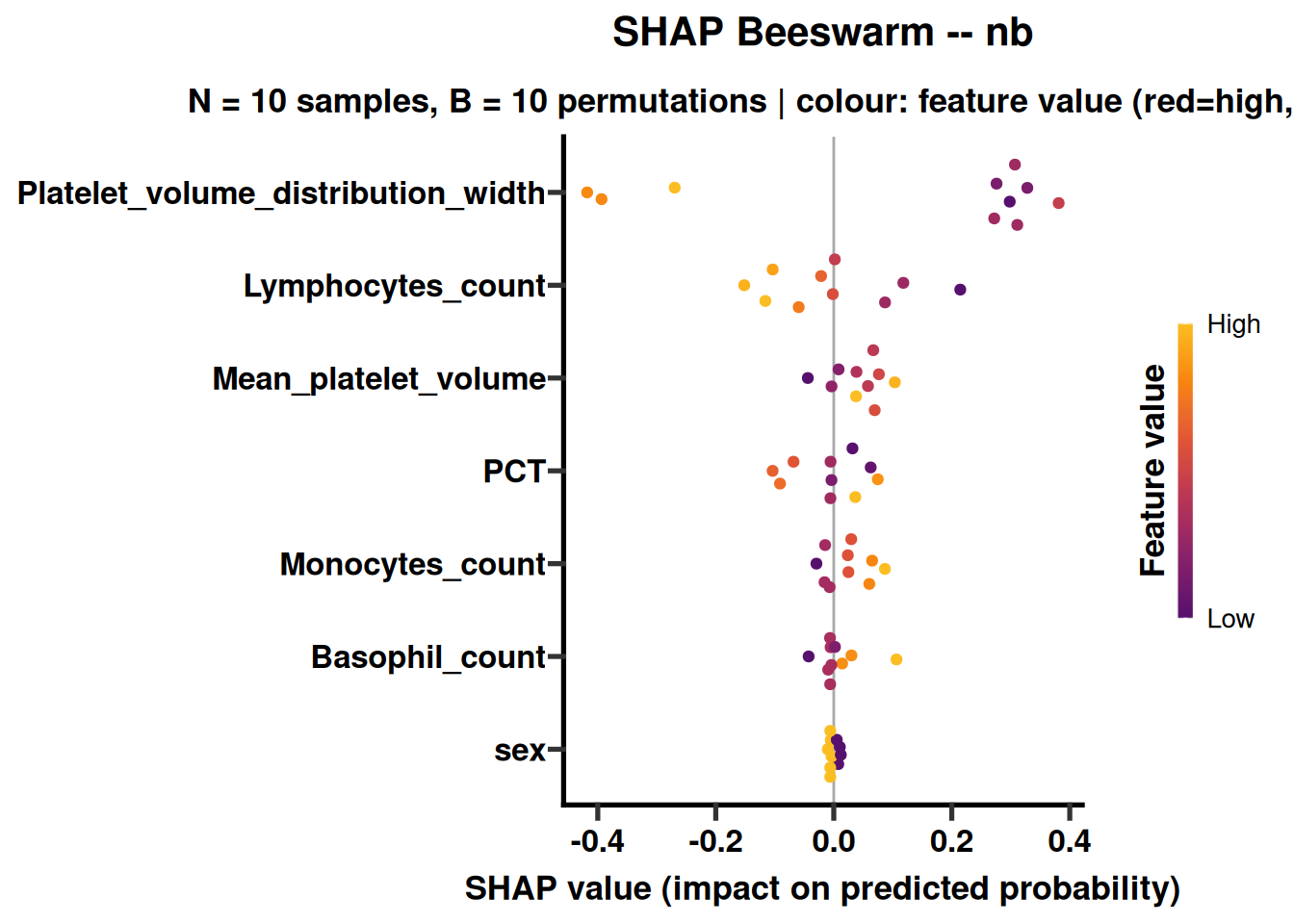
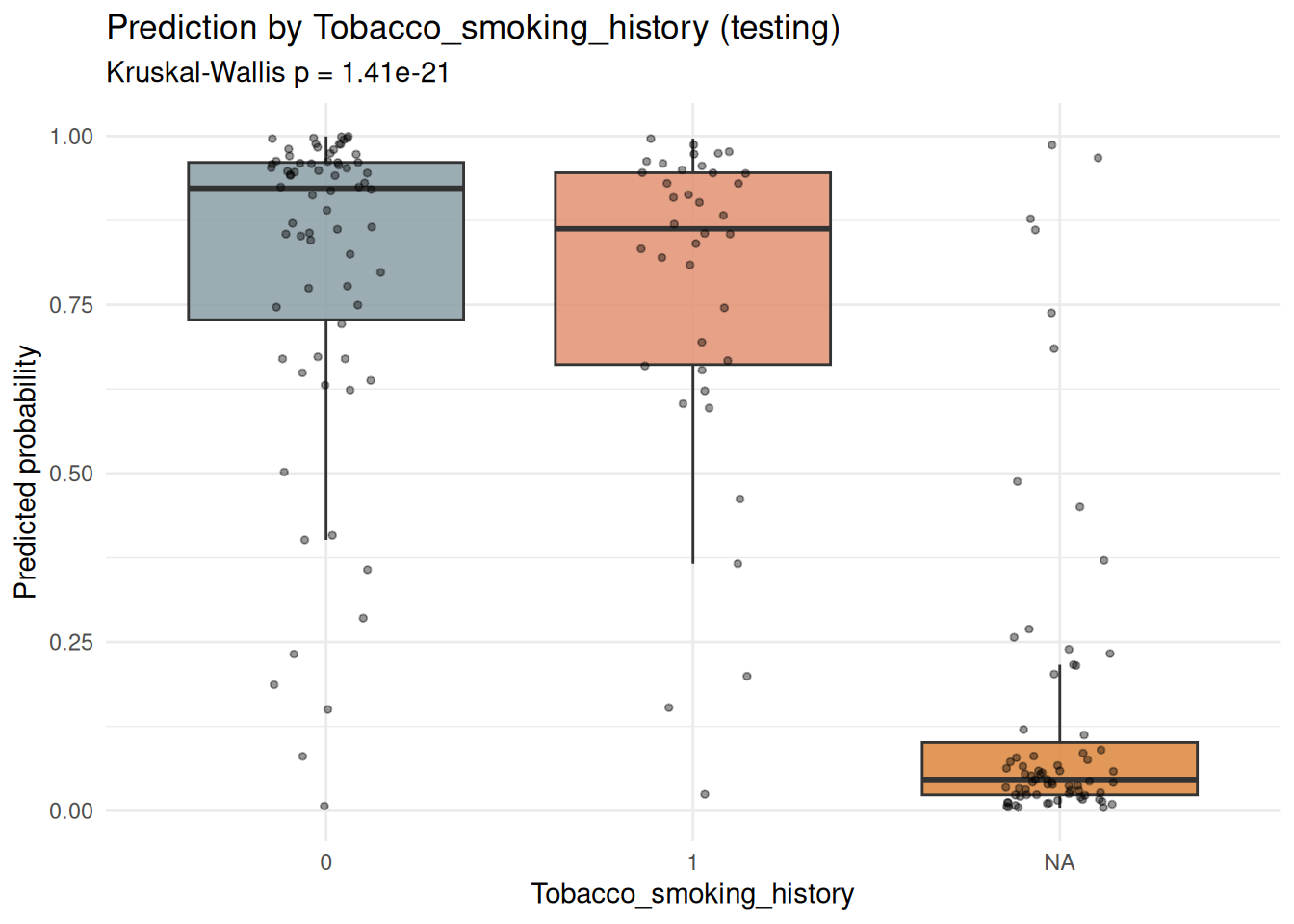
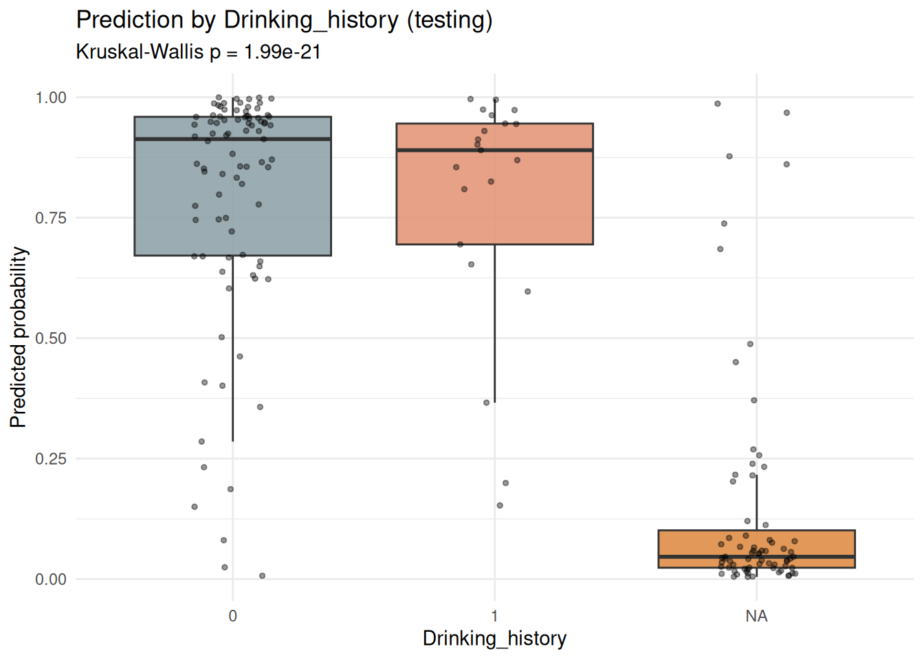
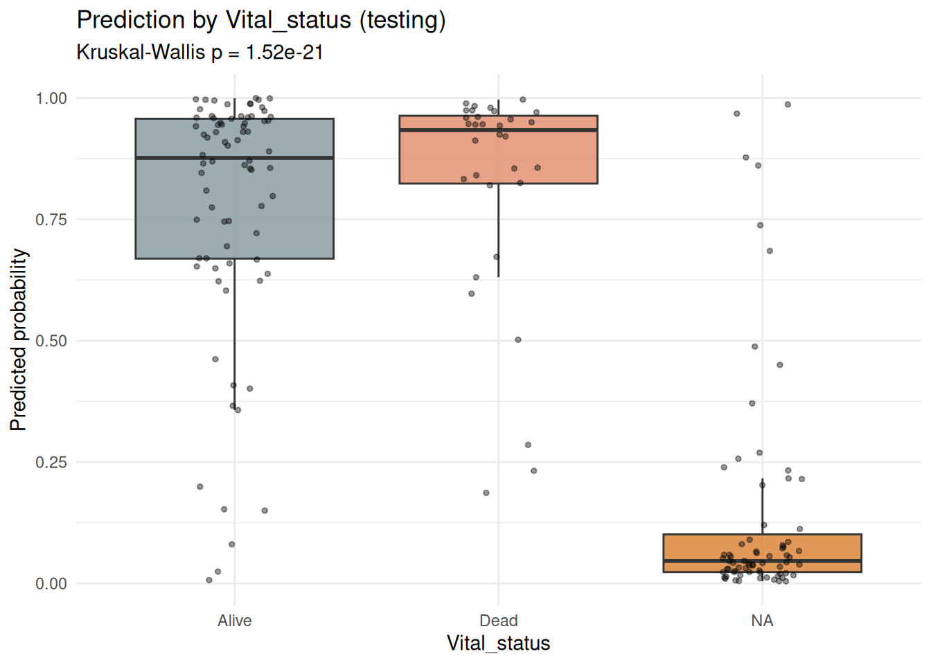
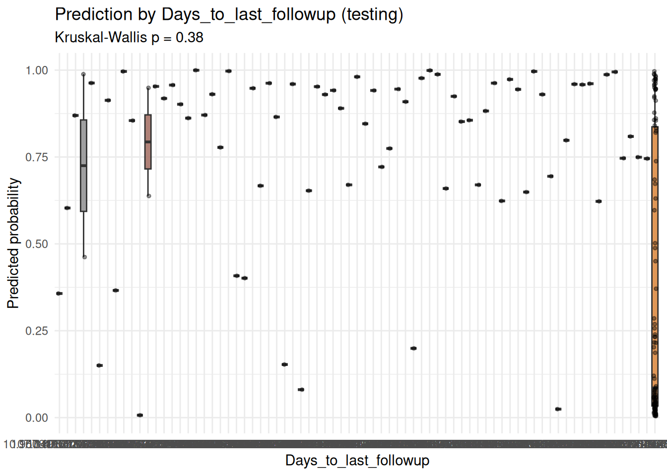
Start by setting `INPUT_STAT_OBJ`, the outcome definition, and `OUTPUT_DIR`. Optional packages are loaded only by the methods that need them. Treat apparent performance from feature selection, tuning, and model comparison as development evidence until it is confirmed in an untouched cohort; all figures and tables are saved in a structured output tree for that audit.
## Step-by-step Workflow
The workflow is divided into short stages. Each note explains the purpose, key checks, and interpretation limits. Generated plots and tables appear directly below their code chunk.
### About this chapter
**Audience.** Advanced users who want to see (and customize) every stage of building, tuning, explaining, and clinically validating a model.
**Input.** Requires `stat_obj.rds`, produced by Module 1.
The chapter runs end to end as one session:
1. **CONFIG**
2. **Load the Stat Object and Convert it to a Modeling Object**
3. **Algorithm Inspection**
4. **Feature Selection**
5. **Preprocessing Benchmark**
6. **Train / Test Split & Scaling**
7. **Model Training**
8. **Model Comparison Visualizations**
9. **Ensemble Models**
10. **Hyperparameter Tuning of the Best Model**
11. **Tuned vs. Untuned Comparison**
12. **Model Explainability (XAI)**
13. **Clinical Integration**
14. **Deployment**
15. **Save the Final Model Object**
### 0 CONFIG
This section defines seeds, output paths, and dependencies. Update these paths and key parameters first when using new data.
````{r}
#| label: module2-advanced-12
#| echo: true
#| message: false
#| warning: false
#| fig-show: hold
#| out-width: '100%'
# 0. CONFIG
# ---------------------------------------------------------------------------
rm(list = ls())
library(icare)
library(caret)

INPUT_STAT_OBJ <- "stat_obj.rds"                 # produced by Module 1
OUTPUT_DIR     <- "./Module2_Advanced_Output"
SEED           <- 123

dir.create(OUTPUT_DIR, showWarnings = FALSE, recursive = TRUE)
# Register OUTPUT_DIR with the package rather than defining a local sub_dir().
# icare already ships sub_dir(); a local definition shadows it only inside this
# script, so functions INSIDE the package that call sub_dir() themselves would
# still resolve it in the icare namespace and write somewhere else. Calling
# set_output_root() points both this script and the package at the same tree.
set_output_root(OUTPUT_DIR)

# =============================================================================
````
### 1 Load the Stat Object and Convert it to a Modeling Object
This section imports and organizes the data. Check dimensions and variable coding before continuing.
````{r}
#| label: module2-advanced-13
#| echo: true
#| message: false
#| warning: false
#| fig-show: hold
#| out-width: '100%'
# 1. Load the Stat Object and Convert it to a Modeling Object
# =============================================================================
stat_obj <- readRDS(INPUT_STAT_OBJ)

# ConvertObject() re-wraps the cleaned data (`clean.data`) into a
# `Train_Model` object, icare's container for the modeling stage.
model_obj <- ConvertObject(stat_obj, to = "Train_Model")
InspectObject(model_obj)
# The outcome column must be an explicit factor for classification models.
model_obj@clean.df[[model_obj@group_col]] <-
  factor(model_obj@clean.df[[model_obj@group_col]])
cat("Outcome distribution:\n")
print(table(model_obj@clean.df[[model_obj@group_col]]))
set.seed(SEED)
idx <- createDataPartition(model_obj@clean.df[[model_obj@group_col]], p = 0.7, list = FALSE)
model_obj@split.data <- list(
  training = model_obj@clean.df[idx, ],
  testing  = model_obj@clean.df[-idx, ]
)
model_obj_train <- CreateModelObject(
  data      = model_obj@split.data$training,
  group_col = model_obj@group_col
)
InspectObject(model_obj_train)
# =============================================================================
````
### 2 Algorithm Inspection
This section trains and compares candidate models. Select models using discrimination, calibration, stability, and clinical utility together.
````{r}
#| label: module2-advanced-14
#| echo: true
#| message: false
#| warning: false
#| fig-show: hold
#| out-width: '100%'
# 2. Algorithm Inspection
# =============================================================================
# Before picking algorithms, it helps to see what hyperparameters each one
# exposes (via caret) and which ones support built-in variable importance.
# Load data
data(allmodel)
df1=allmodel
# List all presets
df2=list_presets()
# Get all linear models
models_of_interest <- get_models(preset = "core")

cat("\n--- Hyperparameters for candidate models ---\n")
for (m in models_of_interest) {
  info <- caret::getModelInfo(m, regex = FALSE)[[1]]
  cat("\n", m, ":", paste(info$parameters$parameter, collapse = ", "))
}
cat("\n\n--- Built-in variable-importance support ---\n")
print(check_varImp_availability(models_of_interest))
# =============================================================================
````
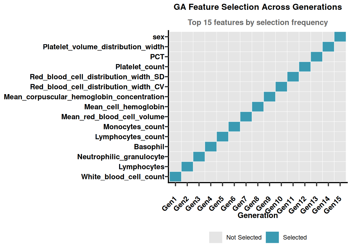
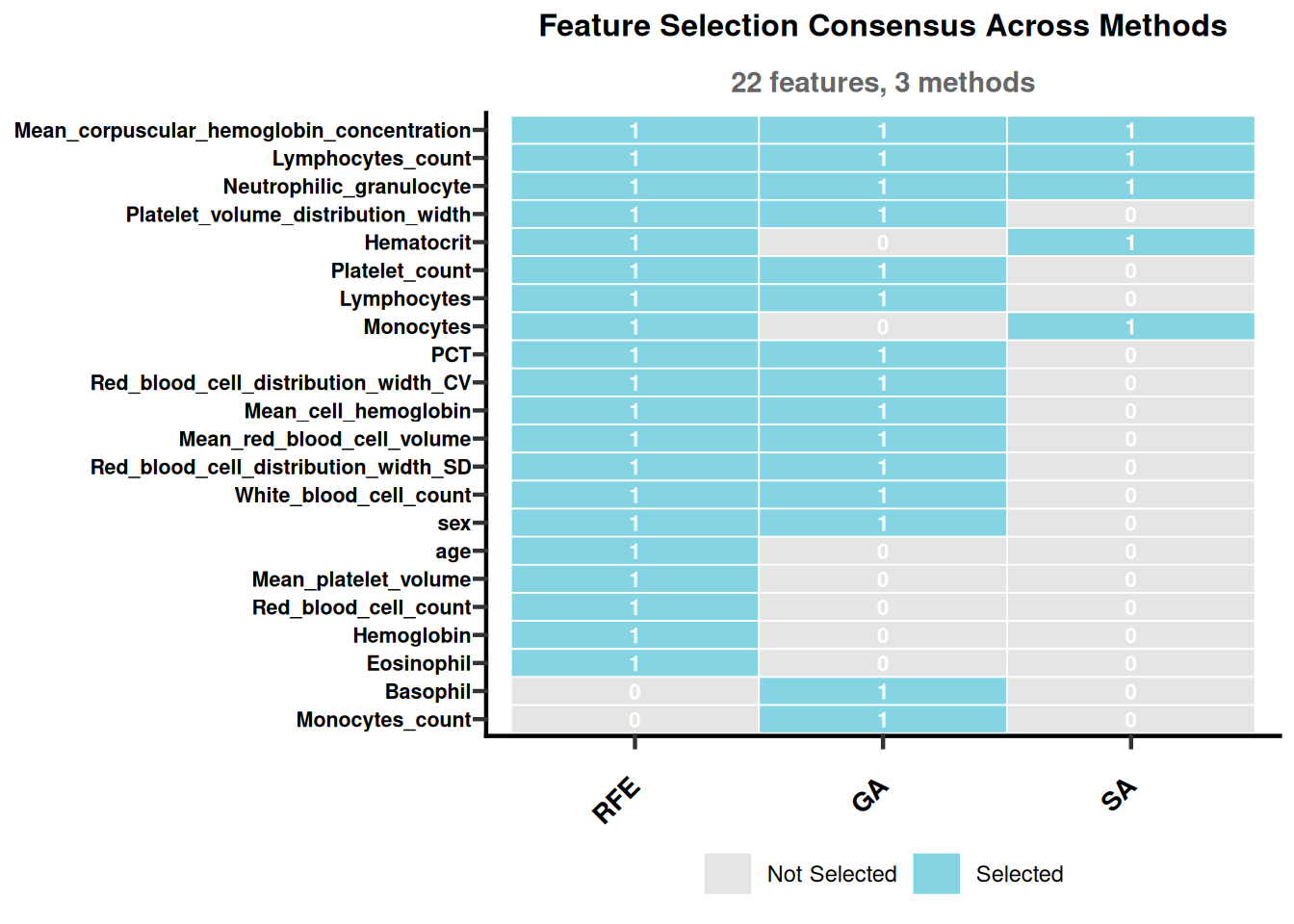
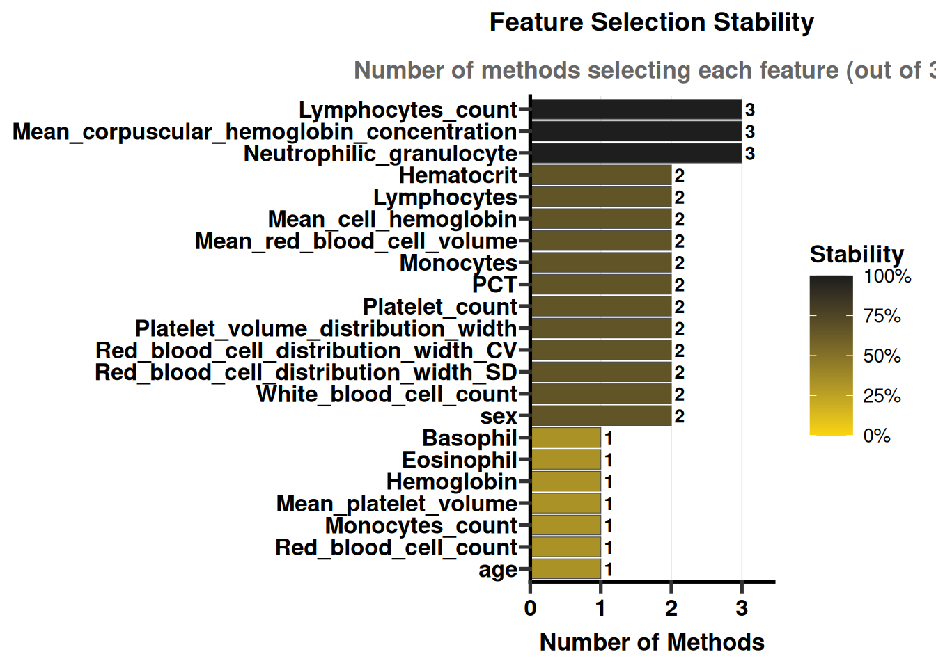
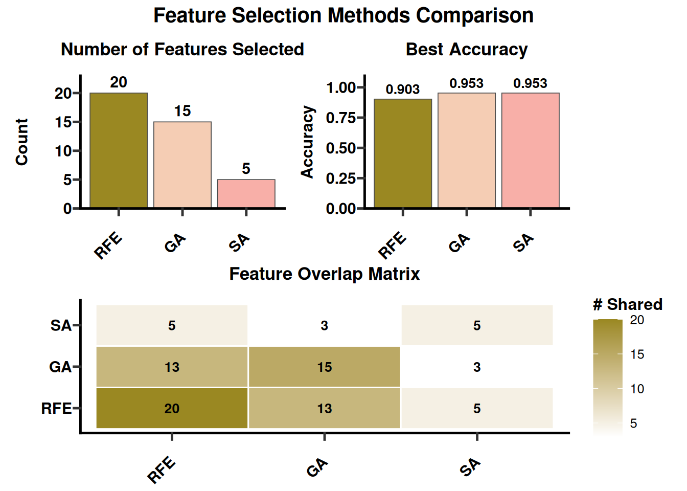
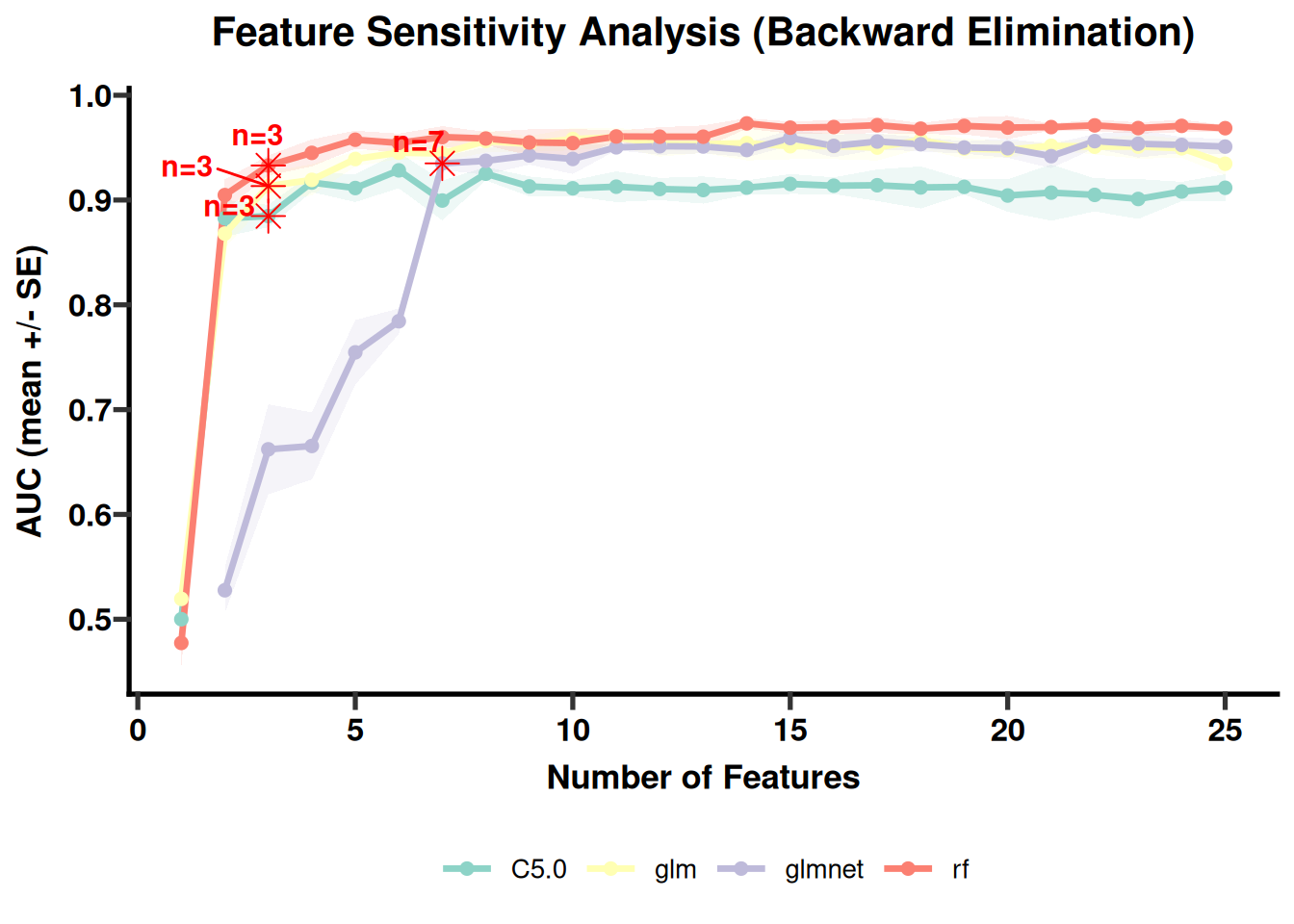
### 3 Feature Selection
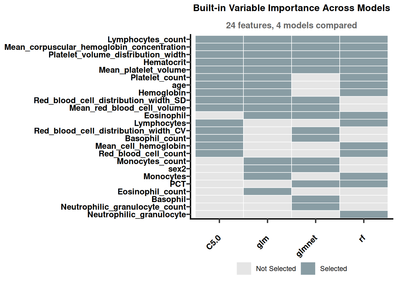
This section selects candidate features. Consider effect size, stability, and biological plausibility rather than a single significance measure.
````{r}
#| label: module2-advanced-15
#| echo: true
#| message: false
#| warning: false
#| fig-show: hold
#| out-width: '100%'
# 3. Feature Selection
# =============================================================================
fs_dir <- sub_dir("01_feature_selection")

## 3.1 Quick pass: built-in importance from a couple of fast models.
## Models that don't support importance are skipped automatically.
builtin <- FeatureSelectBuiltin(
  object = model_obj_train,
  models = models_of_interest,
  top_n  = 15,
  seed   = SEED
)
print(builtin$importance_table)
PlotBuiltinImportance(builtin_result = builtin, save_dir = fs_dir, save_plot = TRUE)
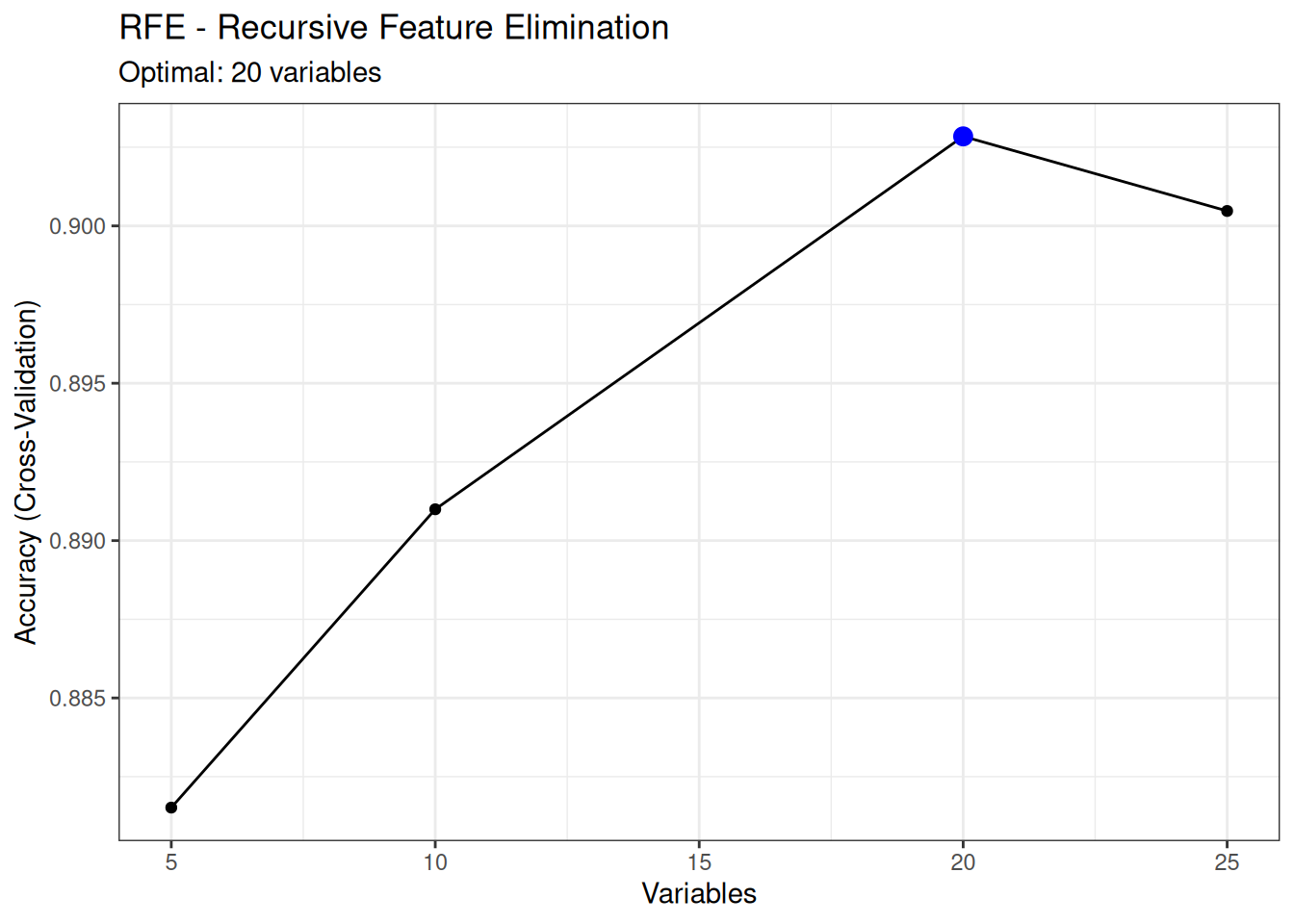
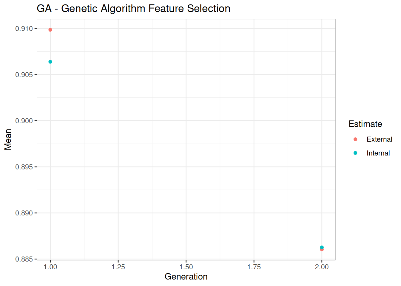
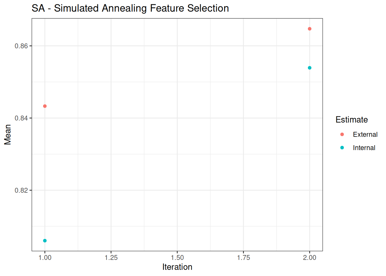
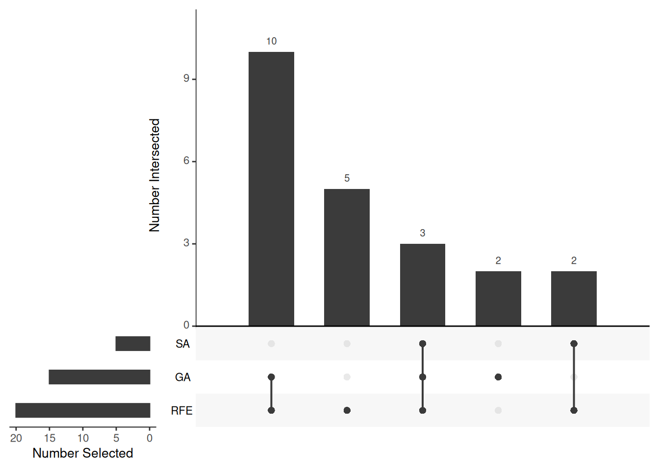
## 3.2 Thorough pass: combine Recursive Feature Elimination (RFE), a Genetic
## Algorithm (GA), and Simulated Annealing (SA), then take the UNION of
## features any method selected. This is slower but more robust than any
## single method — useful when you want a defensible feature set for a paper.
fs <- FeatureSelectionPipeline(
  object    = model_obj_train,
  methods   = c("ga", "rfe", "sa"),
  combine   = "union",
  rfe_args  = list(method = "cv", number = 2, sizes = c(5, 10, 20)),
  sa_args   = list(iters = 2, method = "cv", number = 5, repeats = 1, improve = 3),
  ga_args   = list(ga_func = caret::rfGA, iters = 2, popSize = 5,
                    method = "cv", number = 5,
                    allowParallel = TRUE, genParallel = TRUE),
  upset_plot = TRUE,
  save_plot  = TRUE,
  save_dir   = fs_dir,
  seed       = SEED
)
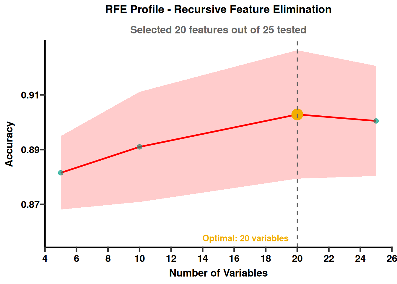
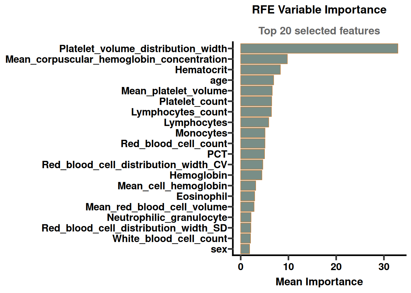
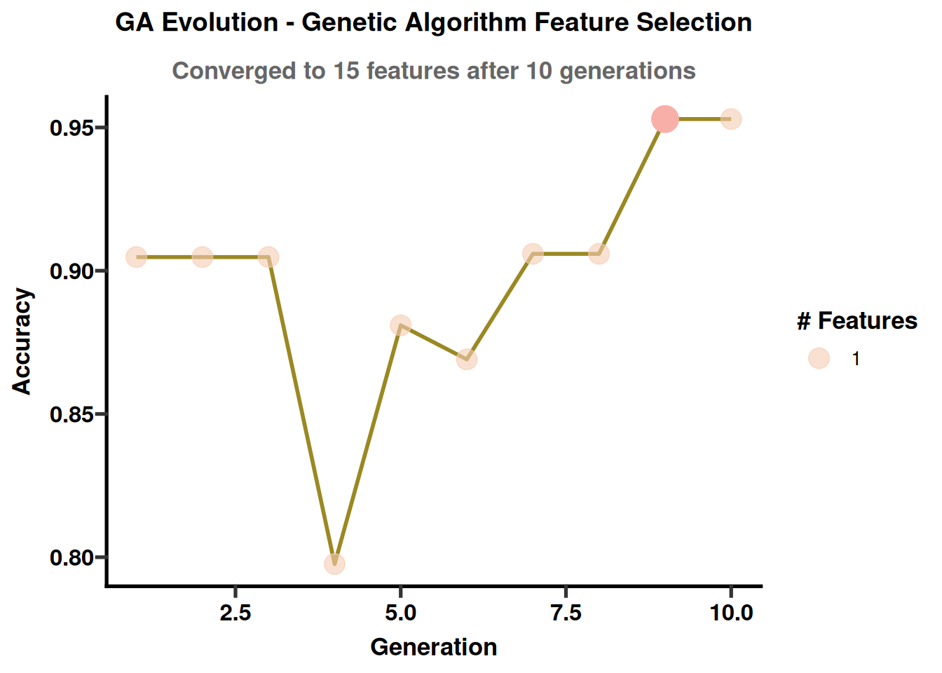
## 3.3 Diagnostic plots for the multi-method feature-selection run.
PlotRFE(fs$results$RFE, metric = "Accuracy", show_optimal = TRUE,y_limits = NULL,
        save_plot = TRUE, save_dir = fs_dir)
PlotRFEImportance(fs$results$RFE, top_n = 20, save_plot = TRUE, save_dir = fs_dir)
PlotGA(fs$results$GA, metric = "Accuracy", save_plot = TRUE, save_dir = fs_dir)
PlotGAFrequency(fs$results$GA, top_n = 30, save_plot = TRUE, save_dir = fs_dir)
PlotFeatureConsensus(fs, show_counts = TRUE, save_plot = TRUE, save_dir = fs_dir)
PlotFeatureStability(fs, top_n = 30, save_plot = TRUE, save_dir = fs_dir,palette_name = 'BottleRocket2')
PlotFeatureComparison(fs, metric = "Accuracy", save_plot = TRUE, save_dir = fs_dir)
## 3.4 A complementary, sensitivity-based approach: train models against an
## increasing number of features, then use an "elbow" rule to find the point
## where adding more features stops helping (either an absolute performance
## tolerance, or a stability window).
elim <- run_feature_elimination(model_obj_train, models = models_of_interest,
                                 number = 5, smooth_span = 0.2)
res_perf   <- select_elbow(elim, "perf_tolerance", tol = 0.05)

plot_elbow(elim, best_features = res_perf$best_features, ci_style = "ribbon",
           save_plot = TRUE, save_dir = fs_dir)

features_perf <- get_selected_features(elim, "perf_tolerance", tol = 0.05)
all_methods   <- get_selected_features(elim, methods = c("perf_tolerance"),
                                        tol = 0.05, window_size = 40, stability_tol = 0.005)

## 3.5 Commit to a final feature set. Here we use the random-forest result
## from the performance-tolerance elbow; swap in `builtin`, `fs$selected`,
## or `all_methods` if you prefer a different method's result.
model_obj_train<- ApplyFeatureSelection(model_obj_train, features_perf$perf_tolerance$best_features$glmnet)
model_obj<- ApplyFeatureSelection(model_obj, features_perf$perf_tolerance$best_features$glmnet)
# =============================================================================
````
### 4 Preprocessing Benchmark
This section preprocesses the data. Review missingness, outlier handling, and normalization before accepting the defaults.
````{r}
#| label: module2-advanced-16
#| echo: true
#| message: false
#| warning: false
#| fig-show: hold
#| out-width: '100%'
# 4. Preprocessing Benchmark
# =============================================================================
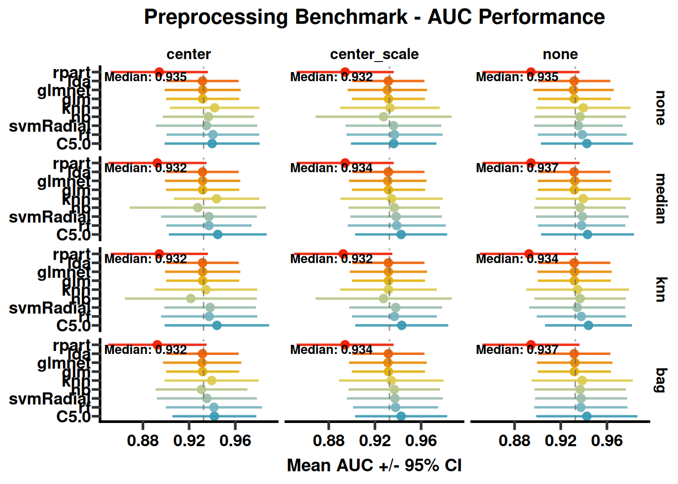
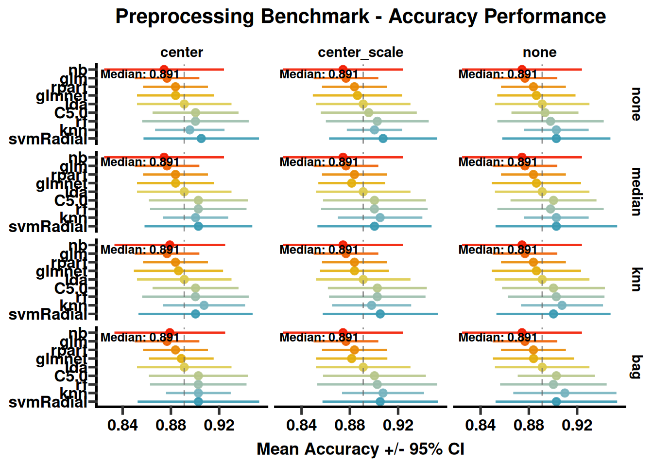
# Before committing to one imputation/normalization recipe, compare a grid of
# (algorithm x imputation x normalization) combinations by cross-validated
# performance. This is optional but strengthens a methods section.
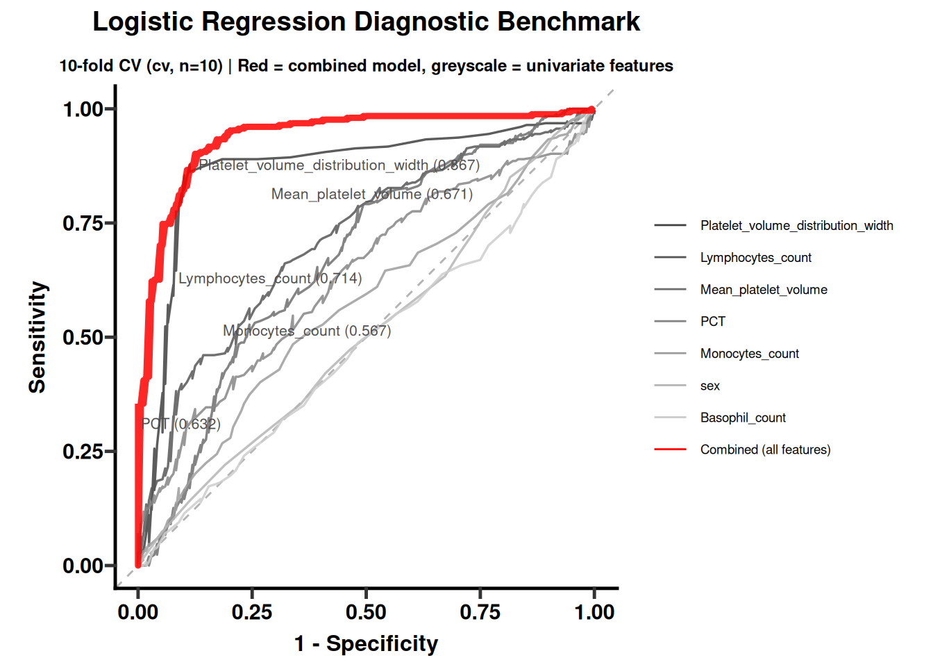
bench <- LogisticDiagnosticBenchmark(
  object = model_obj_train,
  preProcess = c("center", "scale"),
  smote = TRUE,save_plot = TRUE, save_dir = fs_dir)
#algorithms_list=c( 'glm',"lda", "knn","nb","rpart","rf","svmRadial","xgbTree")
algorithms_list=models_of_interest
bench_result <- PreprocessingBenchmark(
  data            = model_obj_train,
  group_col       = model_obj_train@group_col,
  algorithms      = algorithms_list,
  impute_methods  = c("none", "median", "knn", "bag"),
  norm_methods    = list("none", c("center"), c("center", "scale"))
)
print(bench_result)
PlotBenchmarkForest(bench_result, save_plot = TRUE, save_dir =fs_dir,global_median = F)
PlotBenchmarkForest(bench_result, save_plot = TRUE, save_dir =fs_dir,global_median = F,metric = 'Accuracy')
write.csv(bench_result, file.path(fs_dir, "preprocessing_benchmark.csv"), row.names = FALSE)
# =============================================================================
````
### 5 Train / Test Split & Scaling
This section creates training and validation sets. Restrict feature selection and parameter estimation to the training set to prevent leakage.
````{r}
#| label: module2-advanced-17
#| echo: true
#| message: false
#| warning: false
#| fig-show: hold
#| out-width: '100%'
# 5. Train / Test Split & Scaling
# =============================================================================
preProc <- preProcess(
  model_obj@split.data$training[, setdiff(colnames(model_obj@split.data$training), model_obj@group_col)],
  method = c("center", "scale", "YeoJohnson", "bagImpute")
)
model_obj@split.scale.data <- list(
  training = predict(preProc, model_obj@split.data$training),
  testing  = predict(preProc, model_obj@split.data$testing)
)
model_obj@filtered.set <- model_obj@split.scale.data

# =============================================================================
````
### 6 Model Training
This section trains and compares candidate models. Select models using discrimination, calibration, stability, and clinical utility together.
````{r}
#| label: module2-advanced-18
#| echo: true
#| message: false
#| warning: false
#| fig-show: hold
#| out-width: '100%'
# 6. Model Training
# =============================================================================
model_dir <- sub_dir("02_models")

model_obj <- ModelTrainAnalysis(
  object     = model_obj,metric_selection = 'ROC',
  preProcess = NULL,
  tuneLength = 3,
  methods    = models_of_interest,
  control    = list(method = "repeatedcv", number = 5, repeats = 2),
  imbalance_handling = "auto",
  imbalance_threshold = 0.2,
  save_plots = TRUE,
  save_dir   = model_dir,
  seed       = SEED
)
best_row <- model_obj@all.results[which.max(model_obj@all.results$auc), ]
cat("Best model by AUC:", best_row$Model, "\n")
model_obj <- SelectBestModel(model_obj, metric = "auc")
# =============================================================================
````
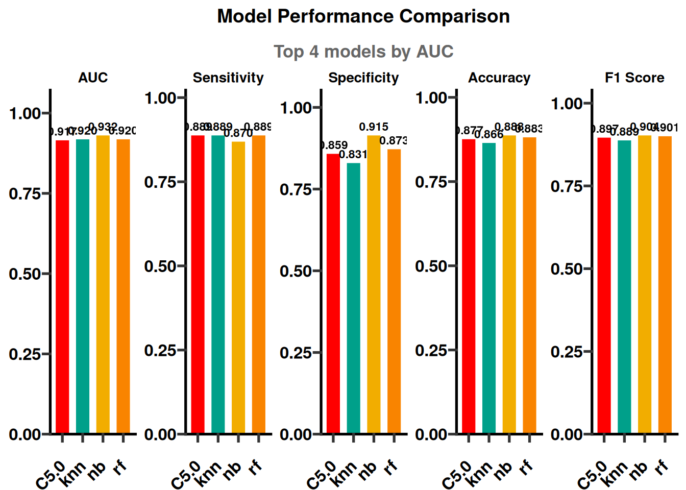
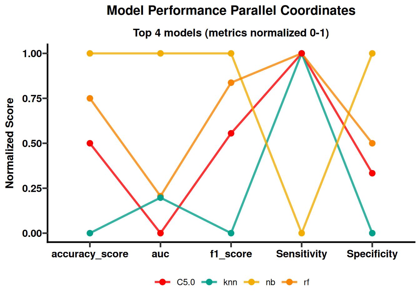
### 7 Model Comparison Visualizations
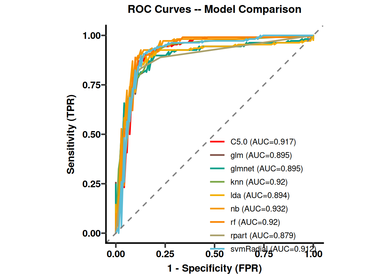
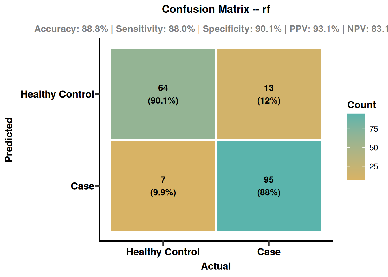
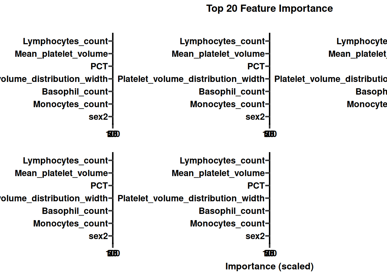
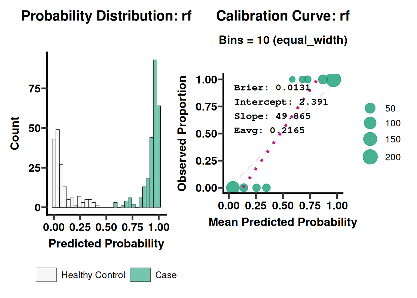
This section trains and compares candidate models. Select models using discrimination, calibration, stability, and clinical utility together.
````{r}
#| label: module2-advanced-19
#| echo: true
#| message: false
#| warning: false
#| fig-show: hold
#| out-width: '100%'
# 7. Model Comparison Visualizations
# =============================================================================
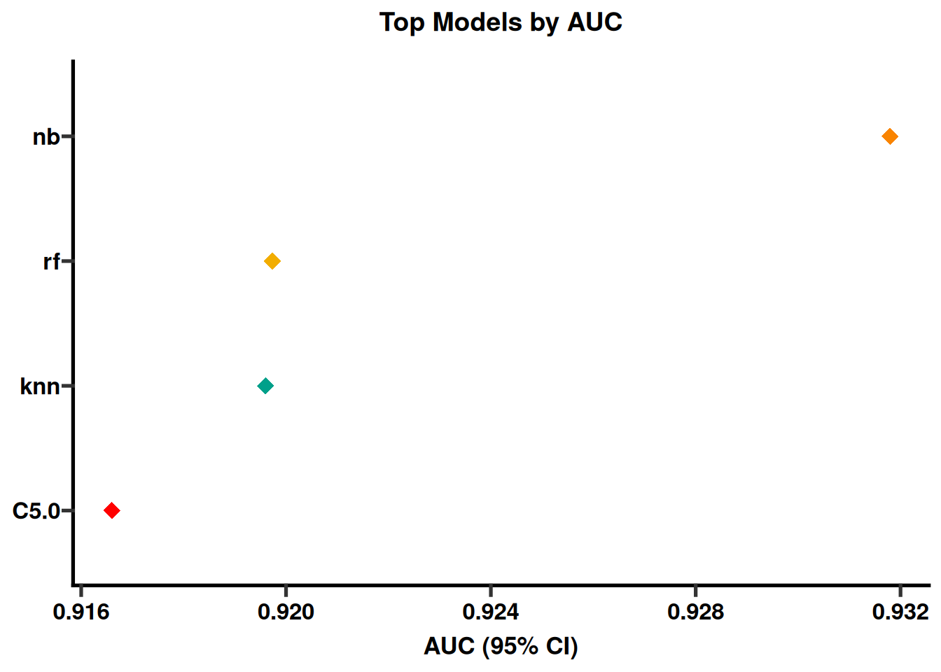
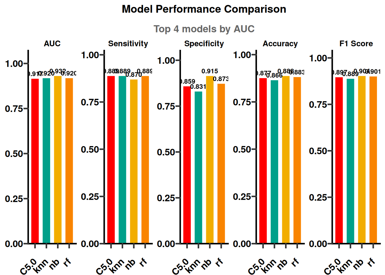
PlotTopModelAUC(model_obj, top_n = 4, save_plot = TRUE, save_dir = model_dir)
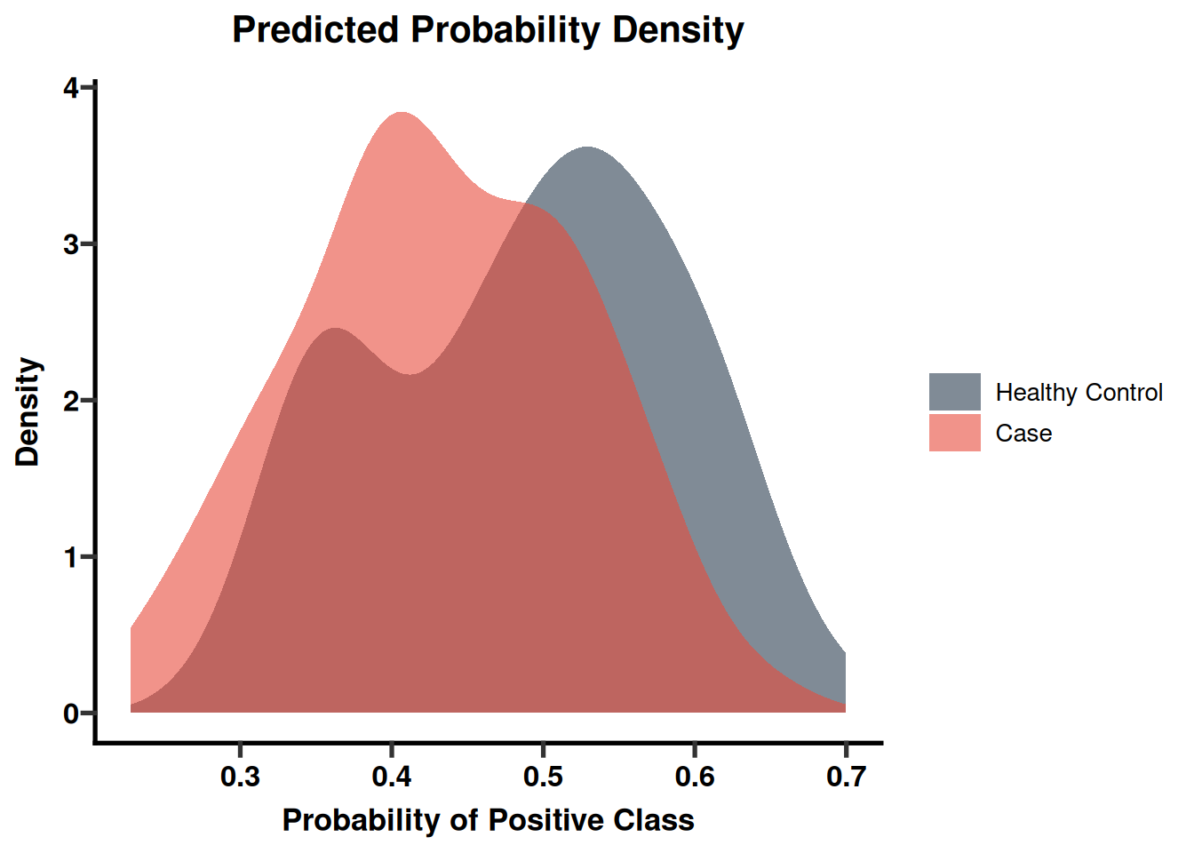
PlotProbDensity(model_obj, save_plot = TRUE, save_dir = model_dir)
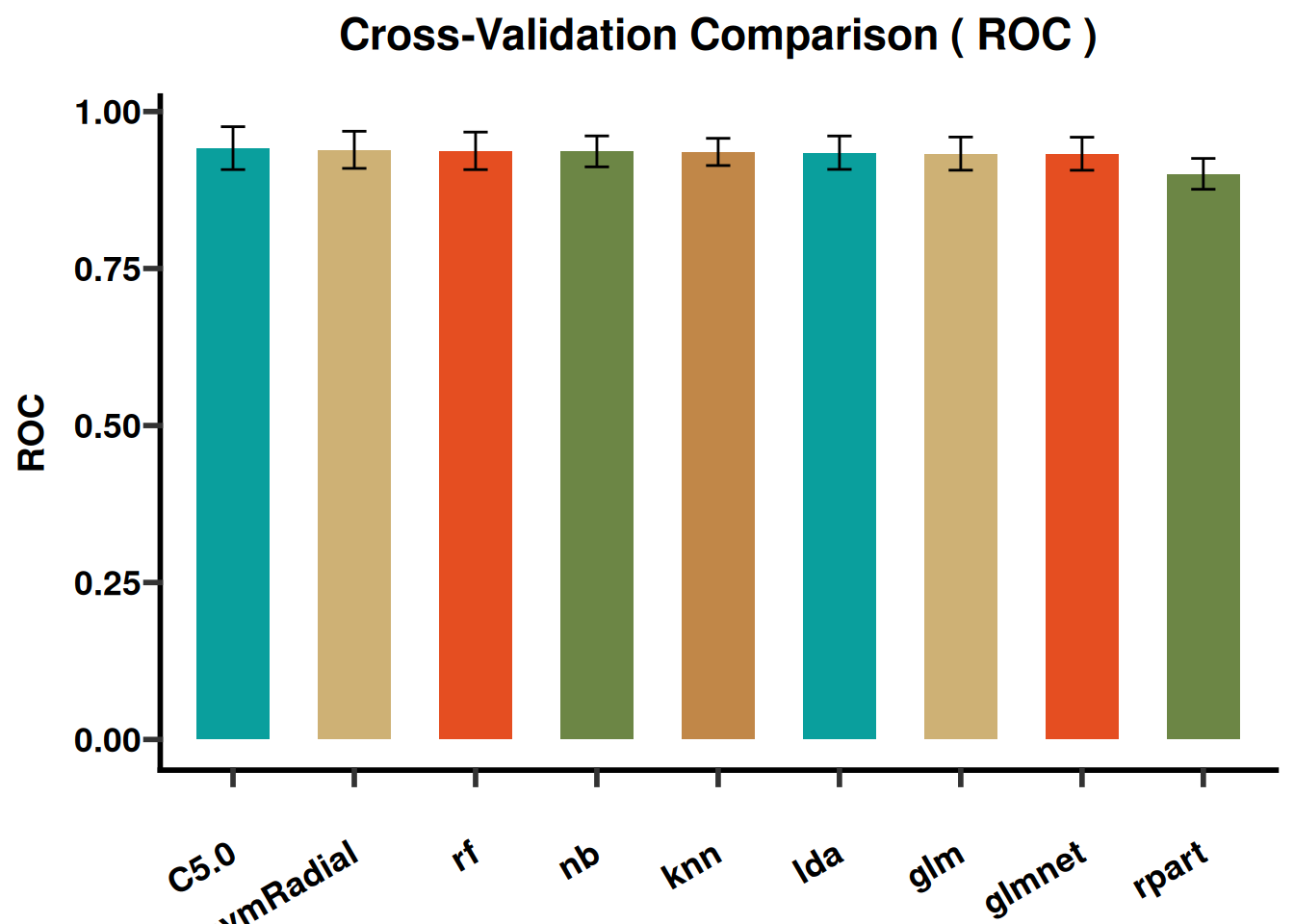
PlotModelComparison(
  model_obj, top_n = 4,
  metrics = c("auc", "Sensitivity", "Specificity", "accuracy_score", "f1_score"),
  palette_name = "Darjeeling1", save_plot = TRUE, save_dir = model_dir,
  width = 12, height = 5
)

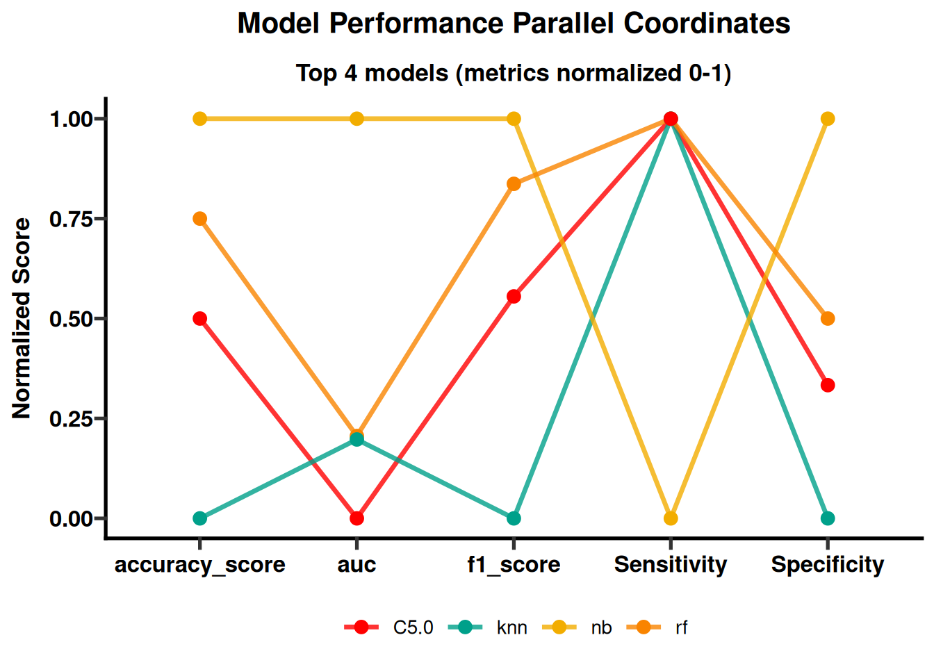
PlotModelParallel(
  model_obj, top_n = 4,
  metrics = c("auc", "Sensitivity", "Specificity", "accuracy_score", "f1_score"),
  save_plot = TRUE, save_dir = model_dir
)
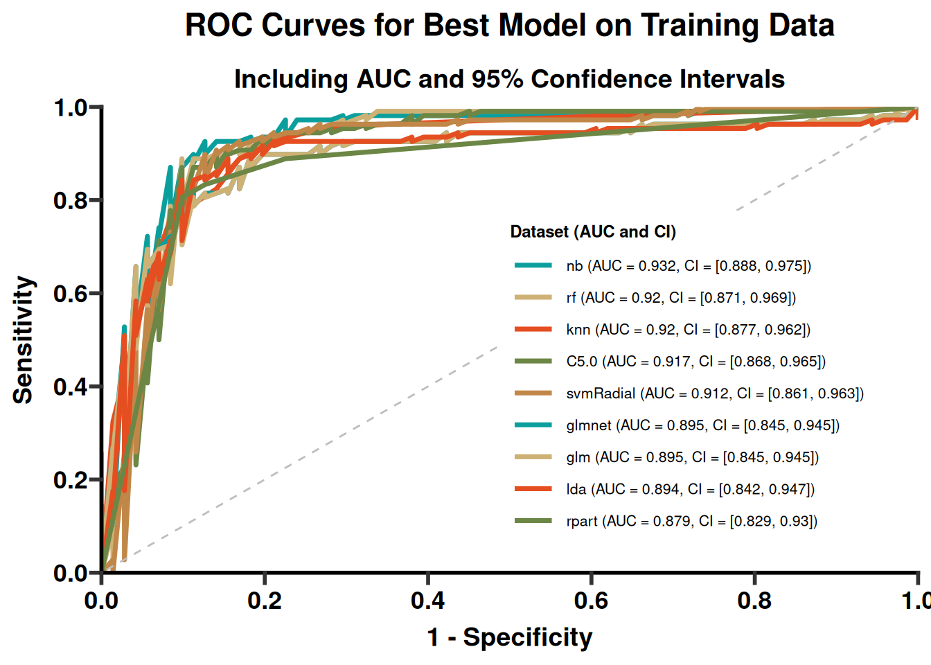
PlotMultiROC(model_obj, test_data = model_obj@split.scale.data$testing,
             palette_name = "Darjeeling1", save_plot = TRUE, save_dir = model_dir)
# Pick a trained model to inspect. "rf" is included in the model list above.
PlotConfusionMatrix(model_obj, test_data = model_obj@split.scale.data$testing,
                    model_name = "rf", threshold = 0.6, prevalence = 0.3,
                    save_plot = TRUE, save_dir = model_dir)
PlotFeatureImportance(model_obj, top_n = 20, save_plot = TRUE, save_dir = model_dir)
PlotCalibration(model_obj, model_name = "rf",
                test_data = model_obj@filtered.set$training,
                save_plot = TRUE, save_dir = model_dir)
PlotCalibration(model_obj, model_name = "rf",
                test_data = model_obj@filtered.set$testing,
                save_plot = TRUE, save_dir = model_dir)
# =============================================================================
````
### 8 Ensemble Models
This section trains and compares candidate models. Select models using discrimination, calibration, stability, and clinical utility together.
````{r}
#| label: module2-advanced-20
#| echo: true
#| message: false
#| warning: false
#| fig-show: hold
#| out-width: '100%'
# 8. Ensemble Models
# =============================================================================
# Train several ensembling strategies on independent copies of model_obj so
# they don't overwrite each other, then compare their held-out AUC.
ens_dir <- sub_dir("03_ensemble")
model_avg    <- TrainEnsemble(model_obj, strategy = "average",  top_n = 4)
model_stack  <- tryCatch(
  TrainEnsemble(model_obj, strategy = "stacking", meta_method = "glm", top_n = 4),
  error = function(e) { message("Stacking unavailable; using average ensemble: ", e$message); model_avg }
)
model_wgt    <- tryCatch(
  TrainEnsemble(model_obj, strategy = "weighted", top_n = 4),
  error = function(e) { message("Weighted ensemble unavailable; using average ensemble: ", e$message); model_avg }
)
model_vote <- TrainEnsemble(model_obj, strategy = "voting", top_n = 4)
# A manually-specified weighting is also supported, e.g. if domain knowledge
# suggests one algorithm should count more than another.
custom_wts   <- c(glm = 0.1, rf = 0.5, gbm = 0.3, svmRadial = 0.1)
model_custom <- tryCatch(
  TrainEnsemble(model_obj, strategy = "weighted", weights = custom_wts, top_n = 4),
  error = function(e) { message("Custom weighting unavailable; using average ensemble: ", e$message); model_avg }
)
test_data <- predict(preProc, model_obj@clean.df)
probs_stack  <- PredictEnsemble(model_stack,  test_data)
probs_avg    <- PredictEnsemble(model_avg,    test_data)
probs_wgt    <- PredictEnsemble(model_wgt,    test_data)
probs_custom <- PredictEnsemble(model_custom, test_data)

library(pROC)
ensemble_auc <- data.frame(
  Strategy = c("Stacking (or Average fallback)", "Average", "Weighted (or Average fallback)", "CustomWeighted (or Average fallback)"),
  AUC = c(
    as.numeric(auc(roc(test_data[[model_obj@group_col]], probs_stack))),
    as.numeric(auc(roc(test_data[[model_obj@group_col]], probs_avg))),
    as.numeric(auc(roc(test_data[[model_obj@group_col]], probs_wgt))),
    as.numeric(auc(roc(test_data[[model_obj@group_col]], probs_custom)))
  )
)
print(ensemble_auc)
write.csv(ensemble_auc, file.path(ens_dir, "ensemble_auc_comparison.csv"), row.names = FALSE)

# Voting returns hard class labels rather than probabilities, so it is
# compared separately by accuracy if needed — omitted here for brevity.

model_obj <- SelectBestModel(model_obj, metric = "auc")
cat("Best single model:", model_obj@best.model.result$model_type, "\n")
# =============================================================================
````
### 9 Hyperparameter Tuning of the Best Model
This section trains and compares candidate models. Select models using discrimination, calibration, stability, and clinical utility together.
````{r}
#| label: module2-advanced-21
#| echo: true
#| message: false
#| warning: false
#| fig-show: hold
#| out-width: '100%'
# 9. Hyperparameter Tuning of the Best Model
# =============================================================================
# --- Reference only: manual, algorithm-specific tuning bounds -------------
# The block below is NOT executed (if (FALSE)). It documents how you would
# manually inspect and set search bounds for a few common algorithms, in
# case the automatic bounds picked in the next section don't suit your data.
if (FALSE) {
  InspectHyperParams("rf")
  InspectHyperParams("xgbTree")
  InspectHyperParams("svmRadial")
  InspectHyperParams("glmnet")

  rf_bounds  <- BuildTuningBounds(mtry = c(2, 15))
  gbm_bounds <- BuildTuningBounds(n.trees = c(50, 500), interaction.depth = c(1, 9),
                                   shrinkage = c(0.001, 0.1), n.minobsinnode = c(5, 30))
  xgb_bounds <- BuildTuningBounds(nrounds = c(50, 300), max_depth = c(2, 10),
                                    eta = c(0.01, 0.3), gamma = c(0, 5),
                                    colsample_bytree = c(0.4, 1),
                                    min_child_weight = c(1, 10), subsample = c(0.5, 1))
  svm_bounds <- BuildTuningBounds(sigma = c(0.001, 0.1), C = c(0.1, 10))
}
# ---------------------------------------------------------------------------

# Automatically detect and tune the best-performing algorithm.
best_method <- model_obj@best.model.result$model_type
cat("Best model type:", best_method, "\n")
InspectHyperParams(best_method)
# Tune the detected best model.  Small datasets can occasionally make the
# Gaussian-process optimiser numerically singular; keep the original model in
# that case and label the comparison accordingly instead of stopping the book.
tuning_error <- NULL
run_bayesian_tuning <- FALSE  # enable only after validating a stable search space
if (run_bayesian_tuning) {
  model_obj <- tryCatch(
    FineTuneModel(
      model_obj, method = best_method, use_scaled = TRUE,
      init_points = 10, n_iter = 5, cv_folds = 5, metric = "ROC", seed = SEED
    ),
    error = function(e) {
      tuning_error <<- e
      message("Bayesian tuning unavailable; retaining the original best model: ", e$message)
      model_obj
    }
  )
} else {
  tuning_error <- simpleError("Bayesian tuning skipped for this reproducible run")
  message("Bayesian tuning skipped; retaining the original best model.")
}
if (is.null(tuning_error)) {
  PlotTuningHistory(model_obj, save_plot = TRUE, save_dir = model_dir)
  tuned_model <- model_obj@best.model.result$fine_tuned_model
} else {
  tuned_model <- model_obj@train.models[[best_method]]
}
model_type  <- model_obj@best.model.result$model_type
orig_best   <- model_obj@train.models[[model_type]]

test_data <- model_obj@split.scale.data$testing
if (is.null(test_data)) test_data <- model_obj@split.data$testing
gc <- model_obj@group_col

original_auc <- max(model_obj@all.results$auc[model_obj@all.results$Model == model_type], na.rm = TRUE)
tuned_auc    <- if (is.null(tuning_error)) max(tuned_model$results$ROC, na.rm = TRUE) else original_auc
comparison_label <- if (is.null(tuning_error)) "tuned" else "untuned fallback"
cat(sprintf(">>> Performance comparison for %s — original AUC: %.4f | %s AUC: %.4f\n",
            model_type, original_auc, comparison_label, tuned_auc))
# =============================================================================
````
### 10 Tuned vs. Untuned Comparison
This section performs the core analysis for this stage. Review the output immediately below the code and confirm that data ranges, assumptions, and results match the study design.
````{r}
#| label: module2-advanced-22
#| echo: true
#| message: false
#| warning: false
#| fig-show: hold
#| out-width: '100%'
# 10. Tuned vs. Untuned Comparison
# =============================================================================
if (is.null(tuning_error)) {
  PlotTunedROC(tuned_model, orig_best, test_data, gc, save_plot = TRUE, save_dir = model_dir)
  PlotTunedConfusion(tuned_model, test_data, gc, save_plot = TRUE, save_dir = model_dir)
  PlotTunedCalibration(tuned_model, test_data, gc, save_plot = TRUE, save_dir = model_dir)
} else {
  message("Tuned-versus-untuned plots skipped because tuning did not converge.")
}

# =============================================================================
````
### 11 Model Explainability (XAI)
This section trains and compares candidate models. Select models using discrimination, calibration, stability, and clinical utility together.
````{r}
#| label: module2-advanced-23
#| echo: true
#| message: false
#| warning: false
#| fig-show: hold
#| out-width: '100%'
# 11. Model Explainability (XAI)
# =============================================================================
xai_dir <- sub_dir("04_explainability")

## 11.1 DALEX explainer for the best model, plus performance/importance plots.
explainer <- CreateExplainer(model_obj)
ExplainModelPerformance(explainer, geom = "roc", save_plots = TRUE, save_dir = xai_dir,
                        plot_width = 6, plot_height = 5)
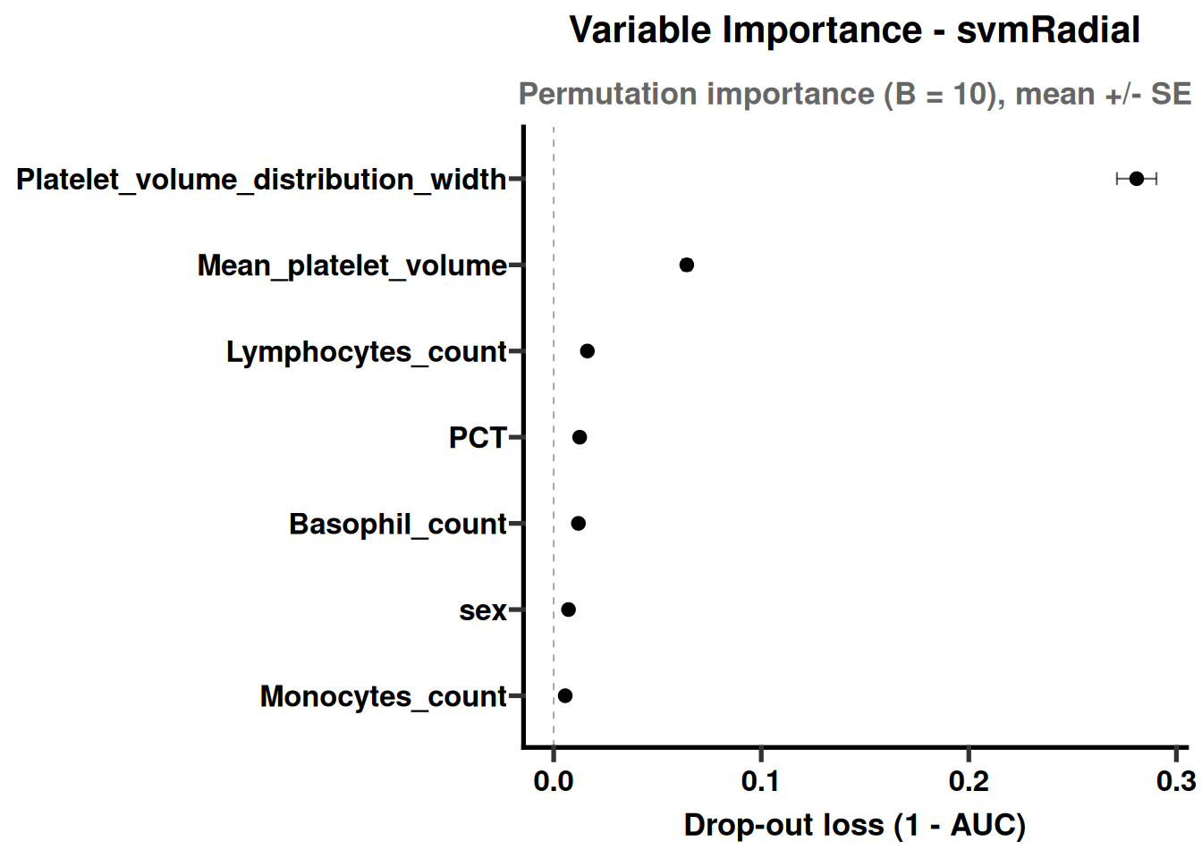
ExplainVariableImportance(explainer, B = 10, top_n = 20, filter_zero = TRUE,
                           save_plots = TRUE, save_dir = xai_dir,
                           plot_width = 8, plot_height = 5)
## 11.2 Global SHAP beeswarm (feature-level contribution across samples).
ExplainSHAPBeeswarm(explainer, N = 10, B = 10, max_features = 8,
                     save_plots = TRUE, save_dir = xai_dir,
                     plot_width = 9, plot_height = 6)
## 11.3 Single-patient explanations for observation #1: waterfall SHAP and
## break-down (which also flags 2-way feature interactions).
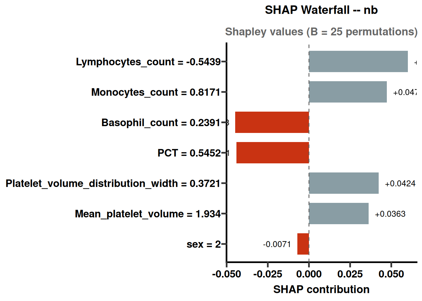
ExplainSHAP(explainer, remove_zero = TRUE, new_observation = 1, B = 25,
            save_plots = TRUE, save_dir = xai_dir, plot_width = 8, plot_height = 5)
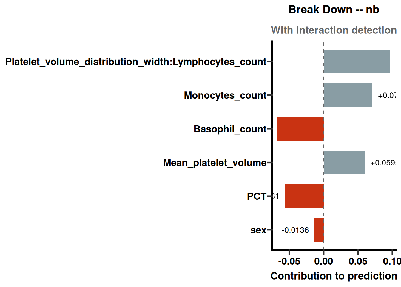
ExplainBreakDown(explainer, remove_zero = TRUE, remove_intercept = TRUE,
                  new_observation = 1, type = "break_down_interactions",
                  save_plots = TRUE, save_dir = xai_dir, plot_width = 8, plot_height = 5)
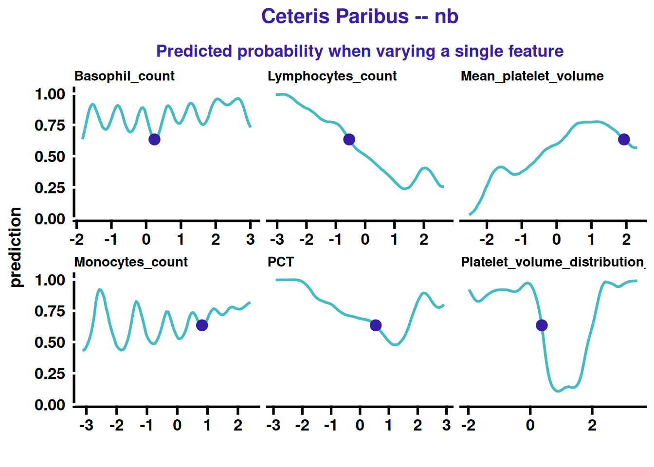
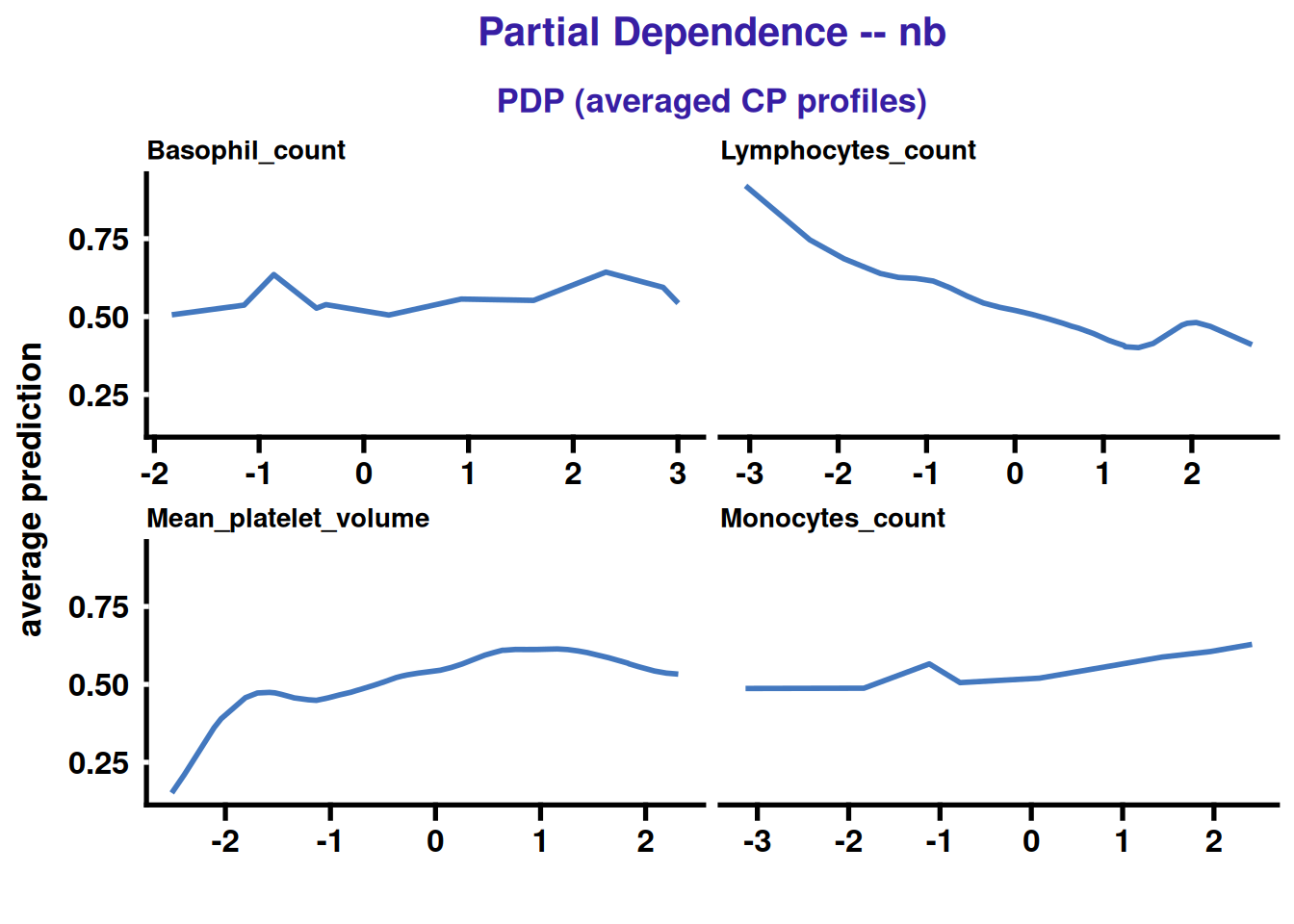
## 11.4 Ceteris-paribus ("what-if") curves and partial-dependence plots.
ExplainCeterisParibus(explainer, new_observation = 1, save_plots = TRUE,
                       save_dir = xai_dir, plot_width = 8, plot_height = 5)
ExplainPartialDependence(explainer, type = "partial", N = 300,
                          save_plots = TRUE, save_dir = xai_dir,
                          plot_width = 8, plot_height = 5)
## 11.5 The same explanations can be generated for any other trained model —
## the un-tuned ensemble, a secondary algorithm, or the fine-tuned model —
## by passing `model =` explicitly.
explainer_gbm <- CreateExplainer(model_obj, model = "svmRadial")
ExplainVariableImportance(explainer_gbm, top_n = 15, save_plots = TRUE,
                           save_dir = file.path(xai_dir, "svmRadial"))
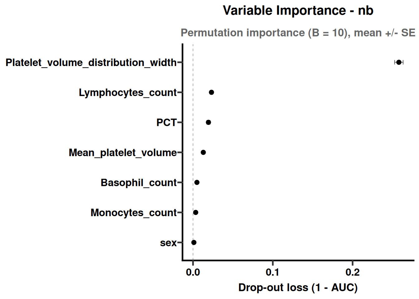
explainer_tuned <- CreateExplainer(model_obj, model = tuned_model)
ExplainVariableImportance(explainer_tuned, top_n = 15, save_plots = TRUE,
                           save_dir = file.path(xai_dir, "tuned"))
model_obj <- tryCatch(
  TrainEnsemble(model_obj, strategy = "stacking", meta_method = "glm", top_n = 4),
  error = function(e) {
    message("Stacking unavailable for XAI; using average ensemble: ", e$message)
    TrainEnsemble(model_obj, strategy = "average", top_n = 4)
  }
)
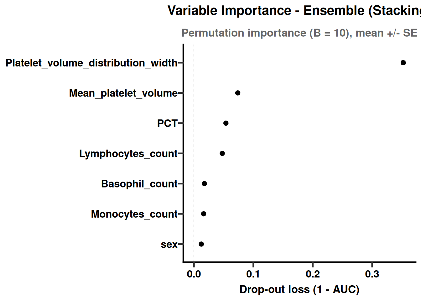
explainer_ens <- CreateExplainer(model_obj, model = "ensemble")
ExplainVariableImportance(explainer_ens, top_n = 15, save_plots = TRUE,
                           save_dir = file.path(xai_dir, "ensemble"))
# =============================================================================
````
### 12 Clinical Integration
This section examines clinical utility and model explanations. Explanatory plots describe model behavior and do not establish causality.
````{r}
#| label: module2-advanced-24
#| echo: true
#| message: false
#| warning: false
#| fig-show: hold
#| out-width: '100%'
# 12. Clinical Integration
# =============================================================================
clin_dir <- sub_dir("05_clinical")

# Attach (here, simulated) clinical covariates that were not part of the
# feature-selected model, for subgroup and confounder analysis.
model_obj@process.info$clinical_data=stat_obj@info.data
df=model_obj@process.info$clinical_data
df=df[,-c(1:4)]
df$Gender=ifelse(df$Gender=='Male',0,1)
df$Lymphocytes_count=model_obj@clean.df$Lymphocytes_count
# CreateStatObject() normalises info.data names (spaces/punctuation -> "_"),
# so the column here is Age_at_diagnosis, not `Age at diagnosis`. Using the
# pre-normalisation name yields NULL, and `NULL > 60` is logical(0): the
# assignment below then fails with "replacement has 0 rows".
df$age_group = ifelse(df$Age_at_diagnosis > 60, '>60 years', '<= 60 years')

model_obj@process.info$clinical_data=df
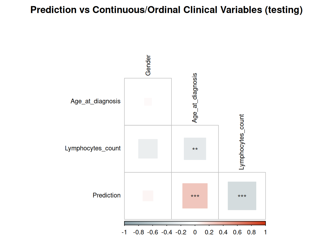
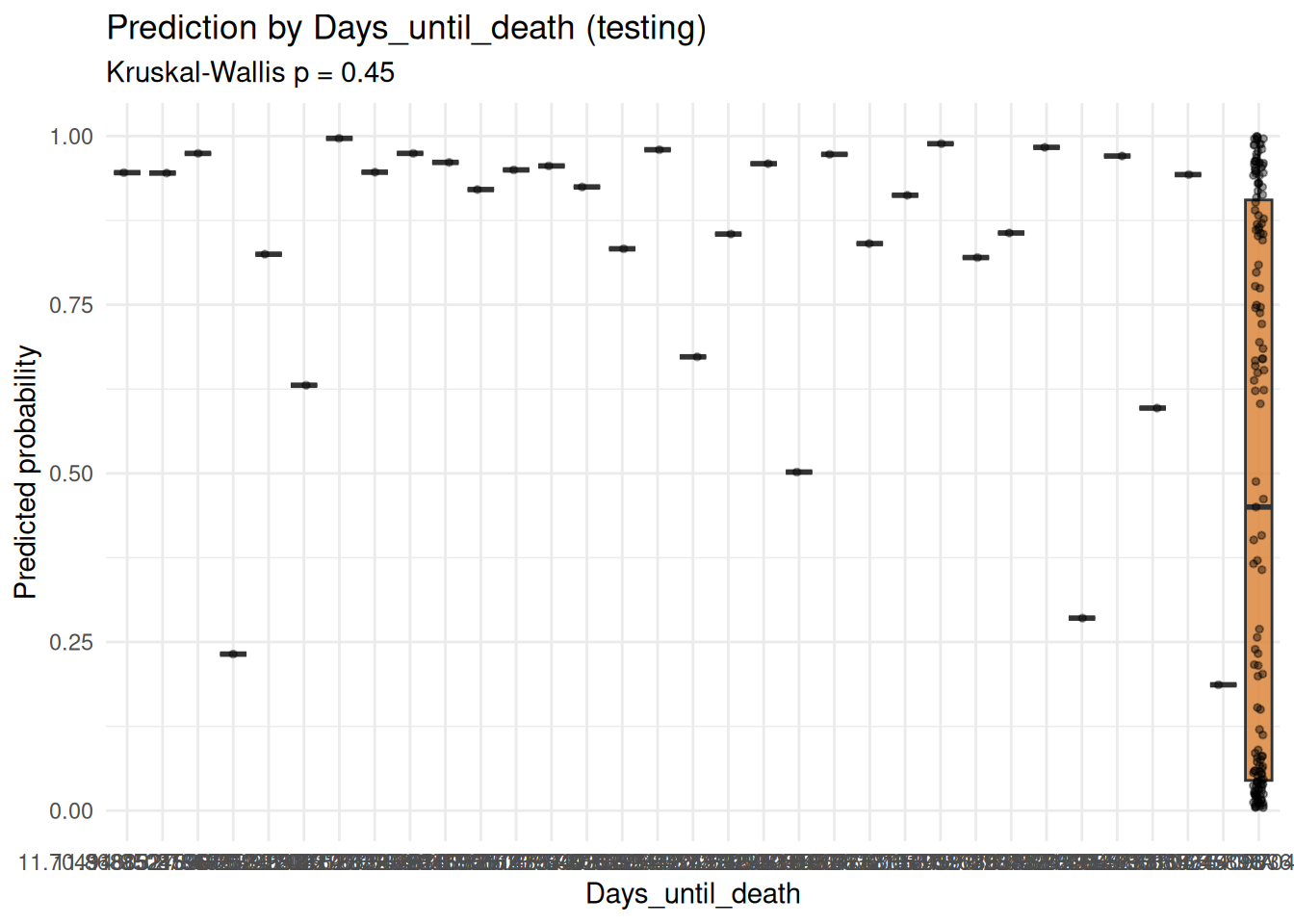
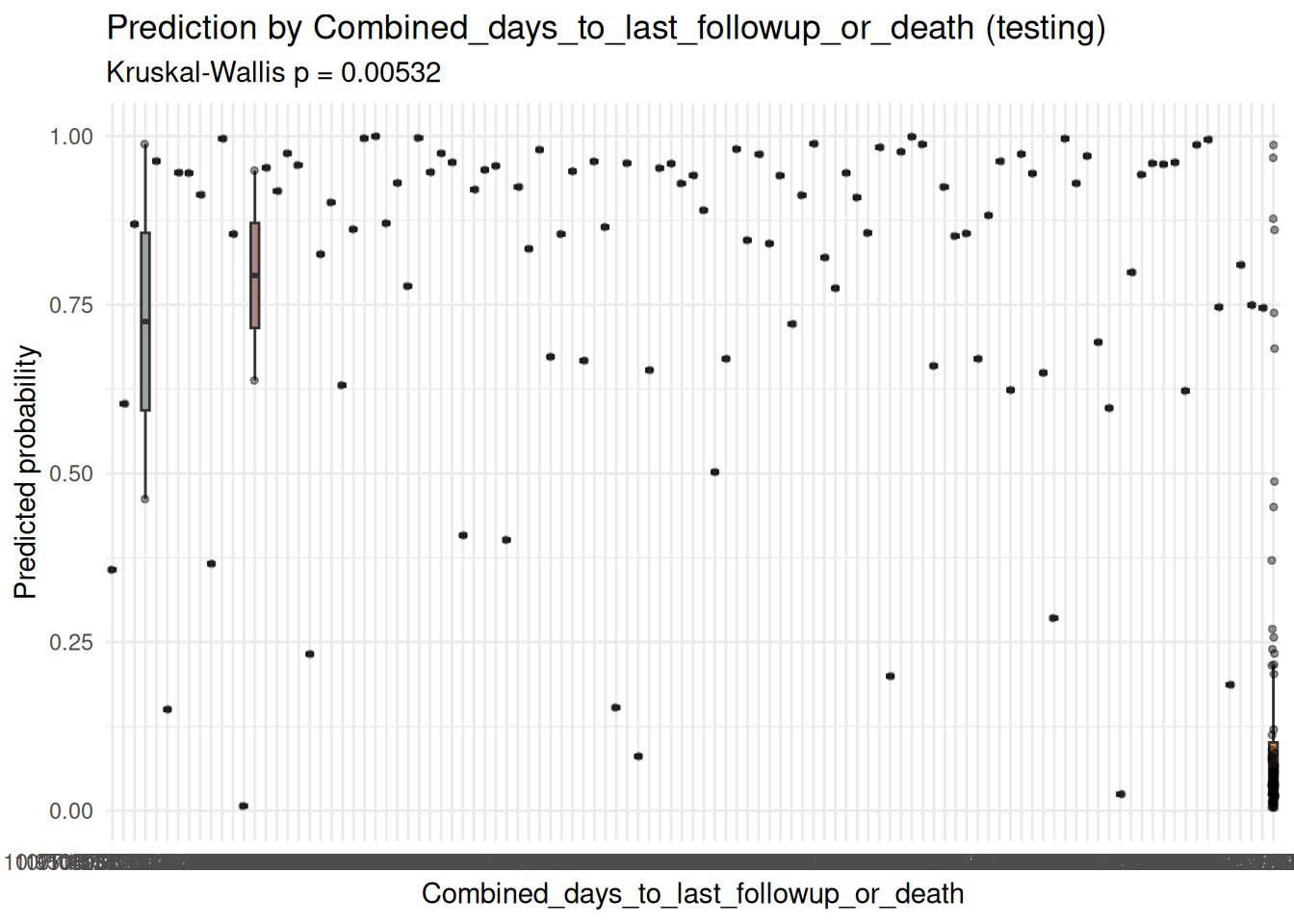
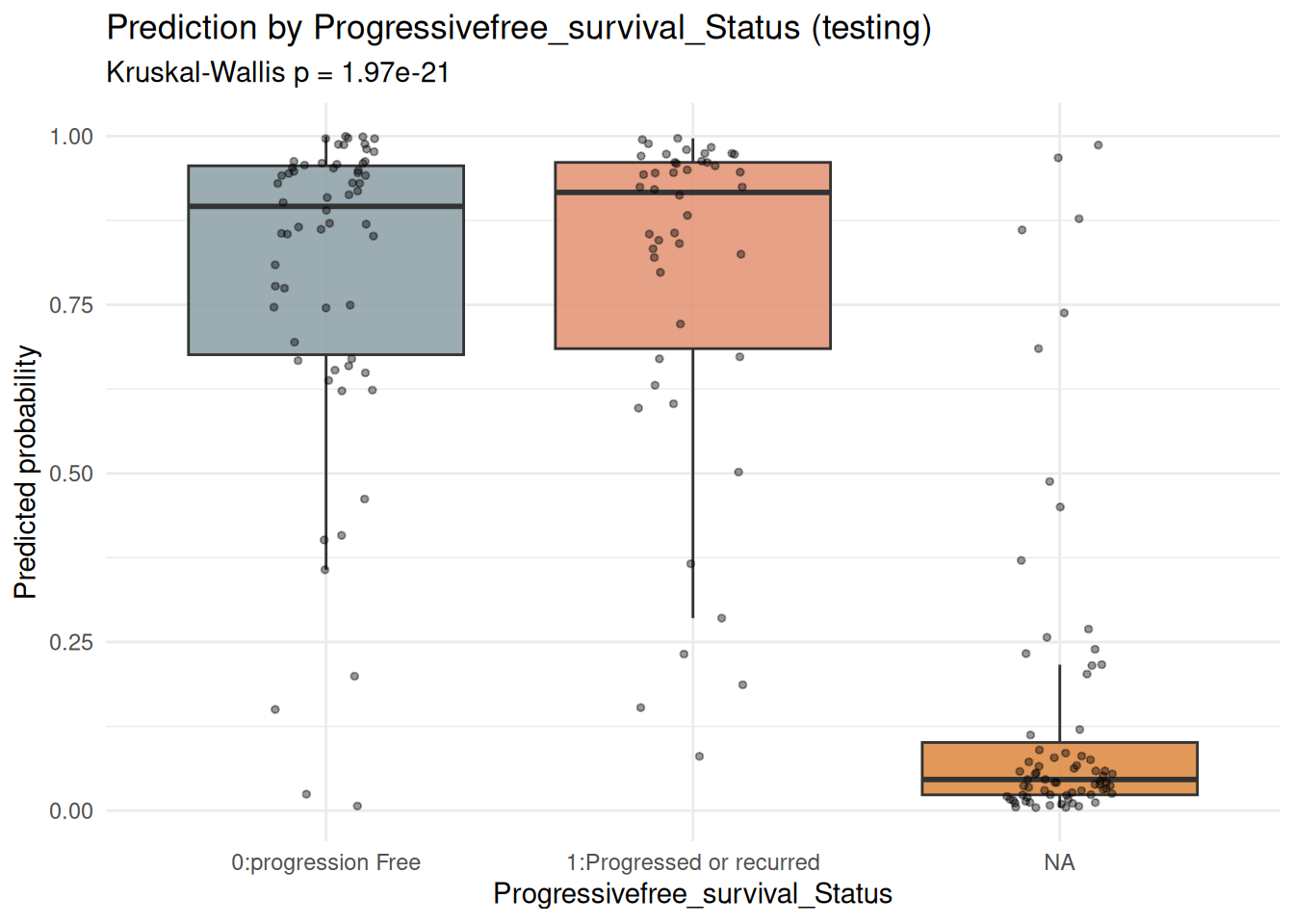
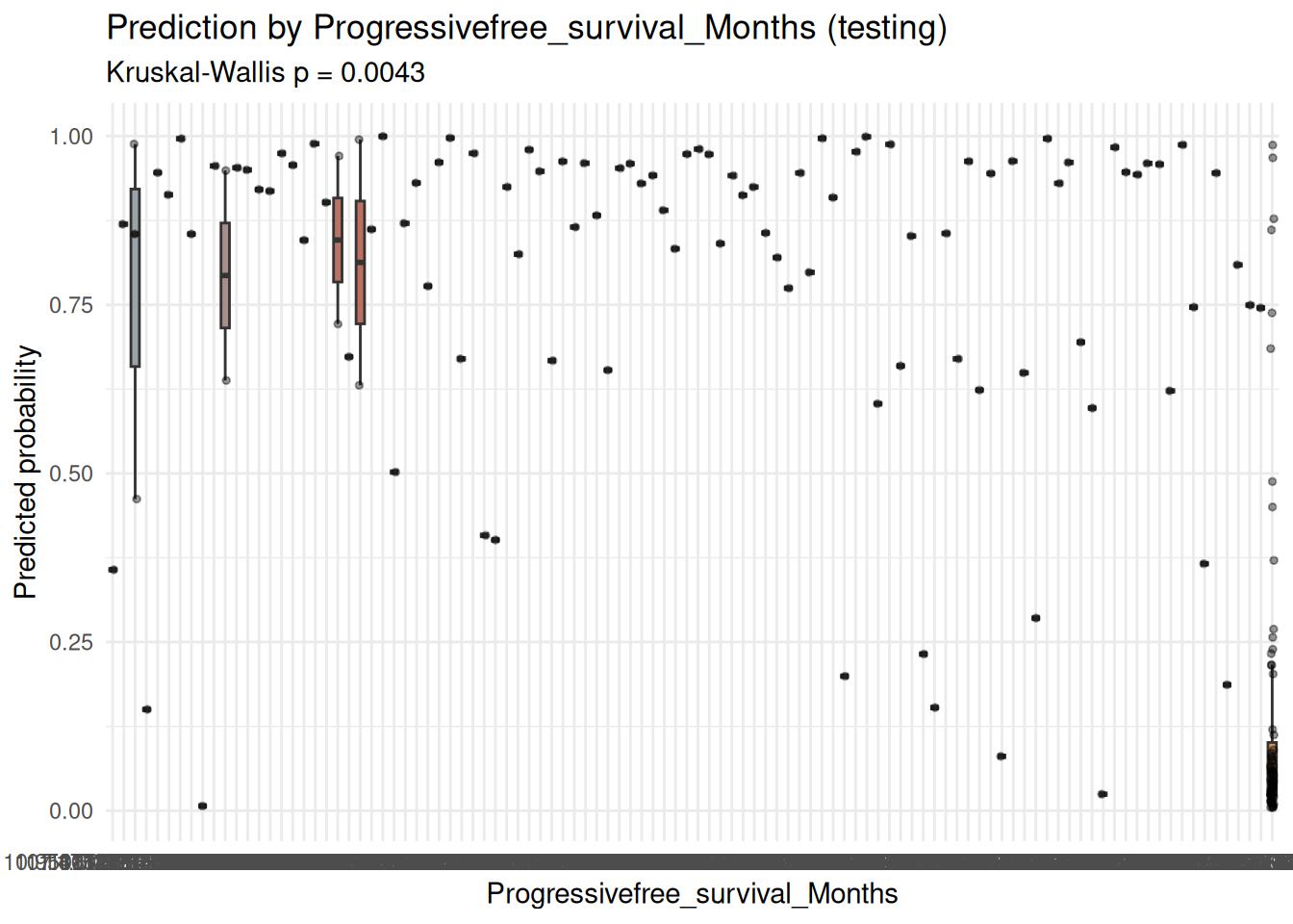
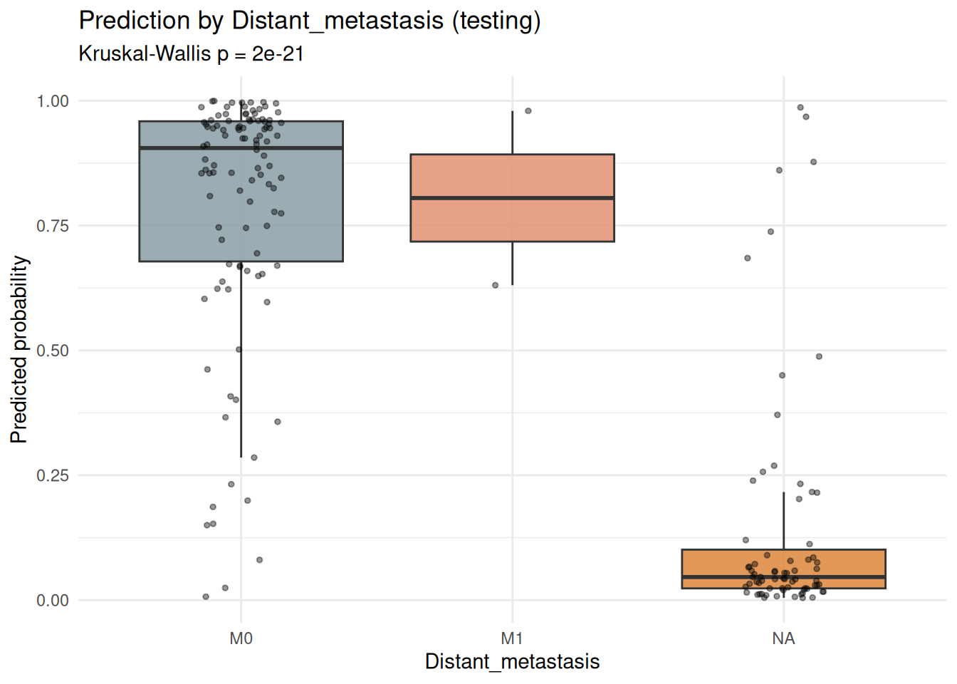
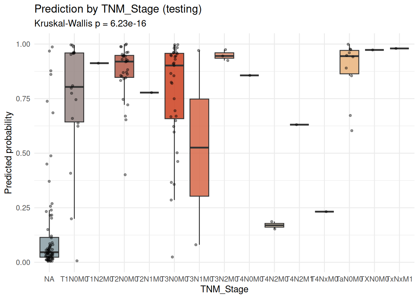
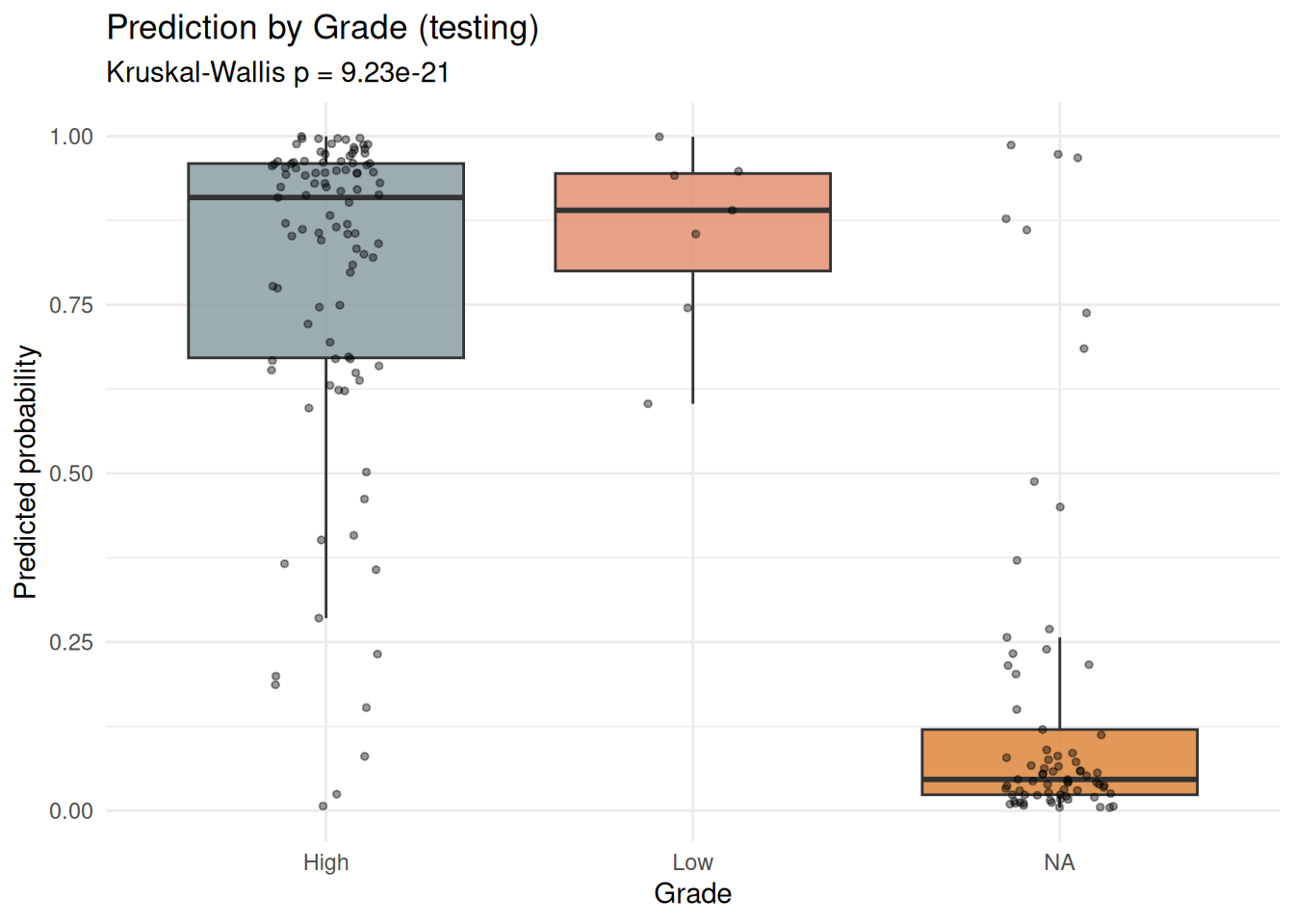
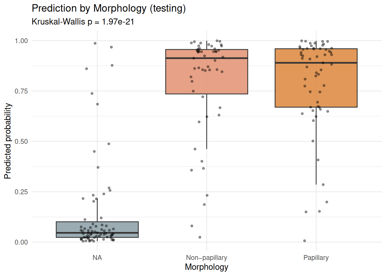
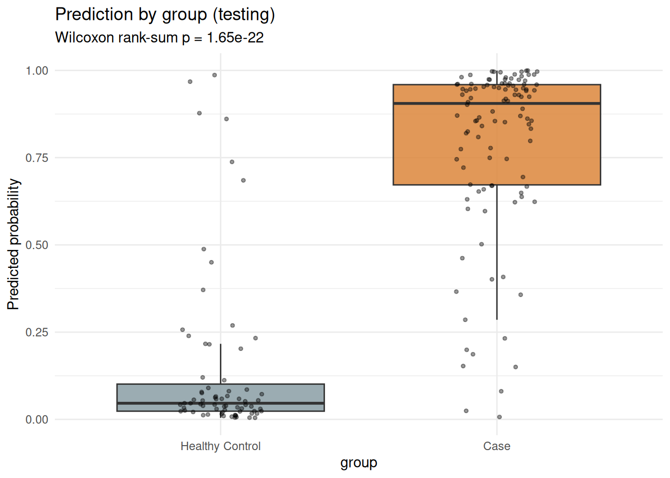
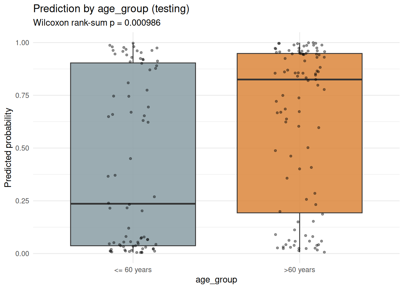
ClinicalCorrelation(model_obj, save_plot = TRUE, save_dir = file.path(clin_dir, "correlation"))
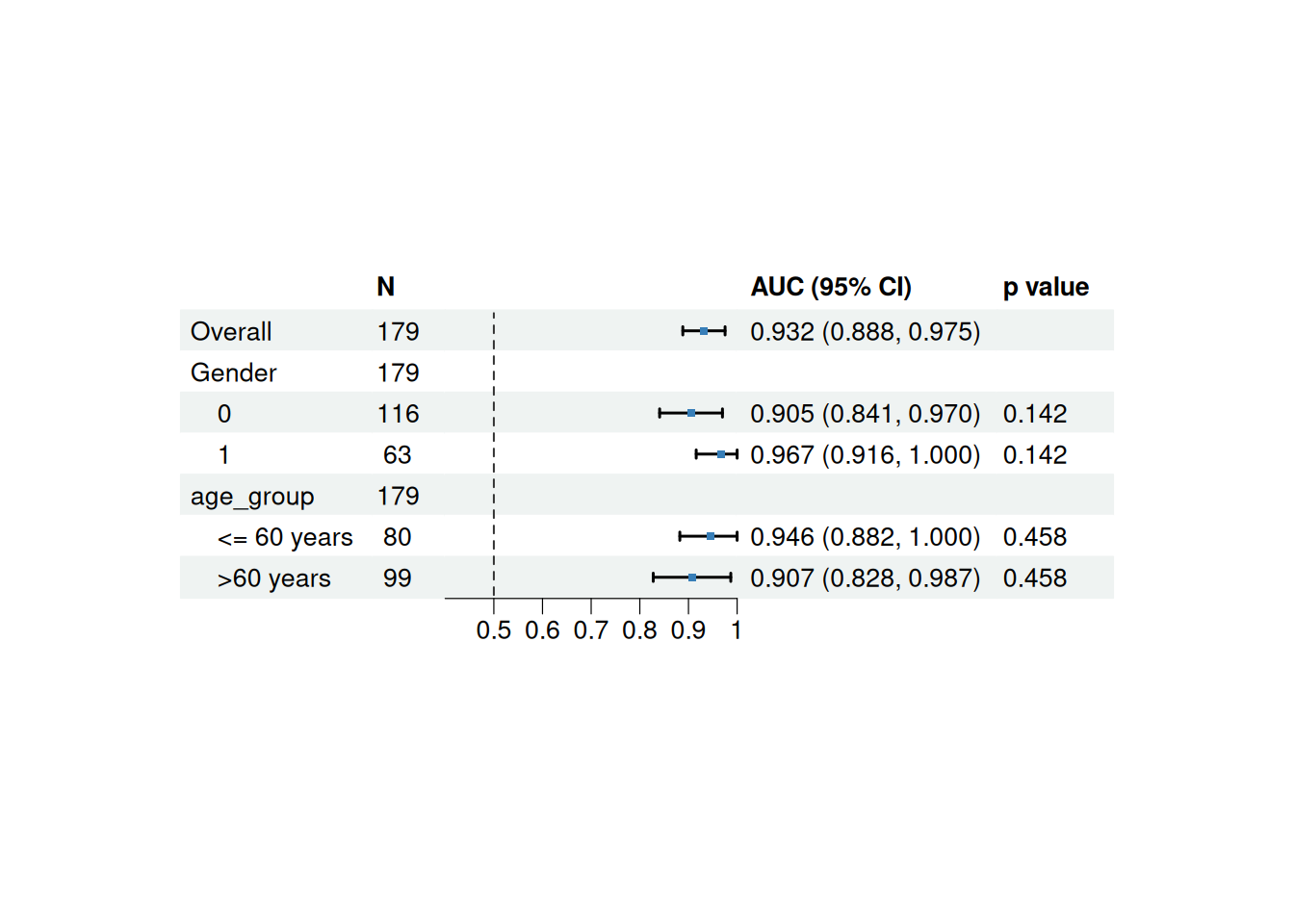
PlotSubgroupForest(model_obj, subgroup_var = c("Gender", "age_group"),compare_method = 'delong_vs_rest',
                    save_plot = TRUE, save_dir = file.path(clin_dir, "subgroup"))
newdata <- model_obj@split.data$testing
model_obj@process.info$clinical_data
# positive_class must name a factor level of the outcome: the label here is
# "Healthy Control" / "Case" (see Module 1), so the events are "Case".
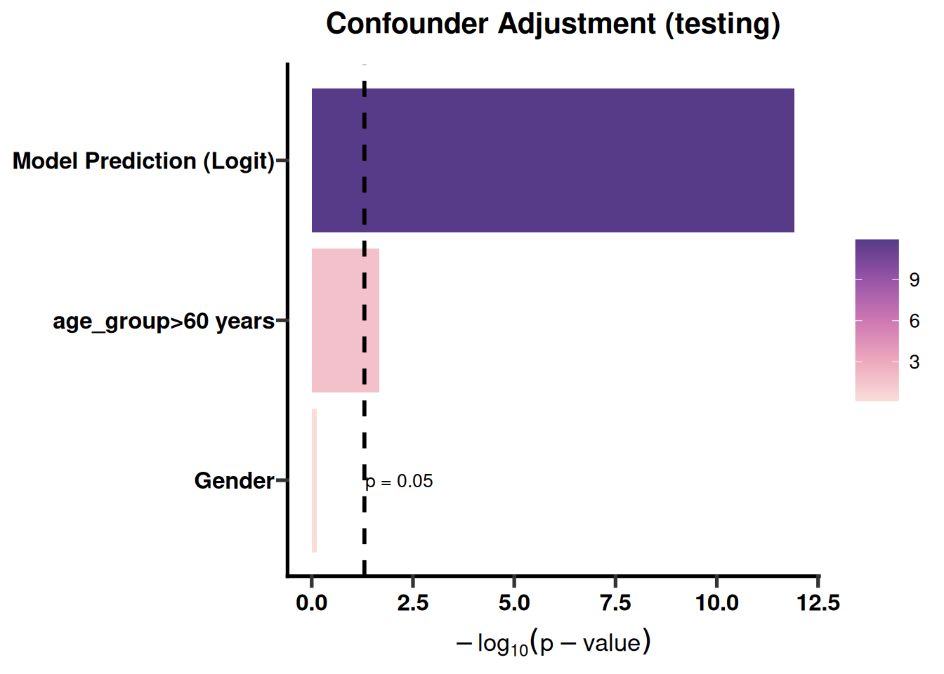
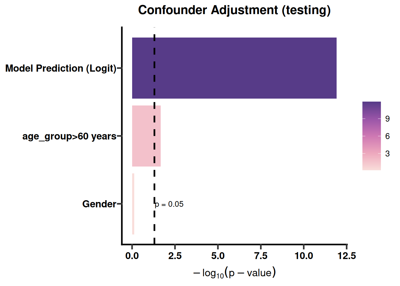
PlotConfounderForest(model_obj, dataset_type = "testing",adjust_vars= c("Gender", "age_group"),outcome_var="group",
                     save_plot = TRUE,positive_class = 'Case', save_dir = file.path(clin_dir, "Confounder"))
# --- 12.1 Decision thresholds for the best model ---------------------------
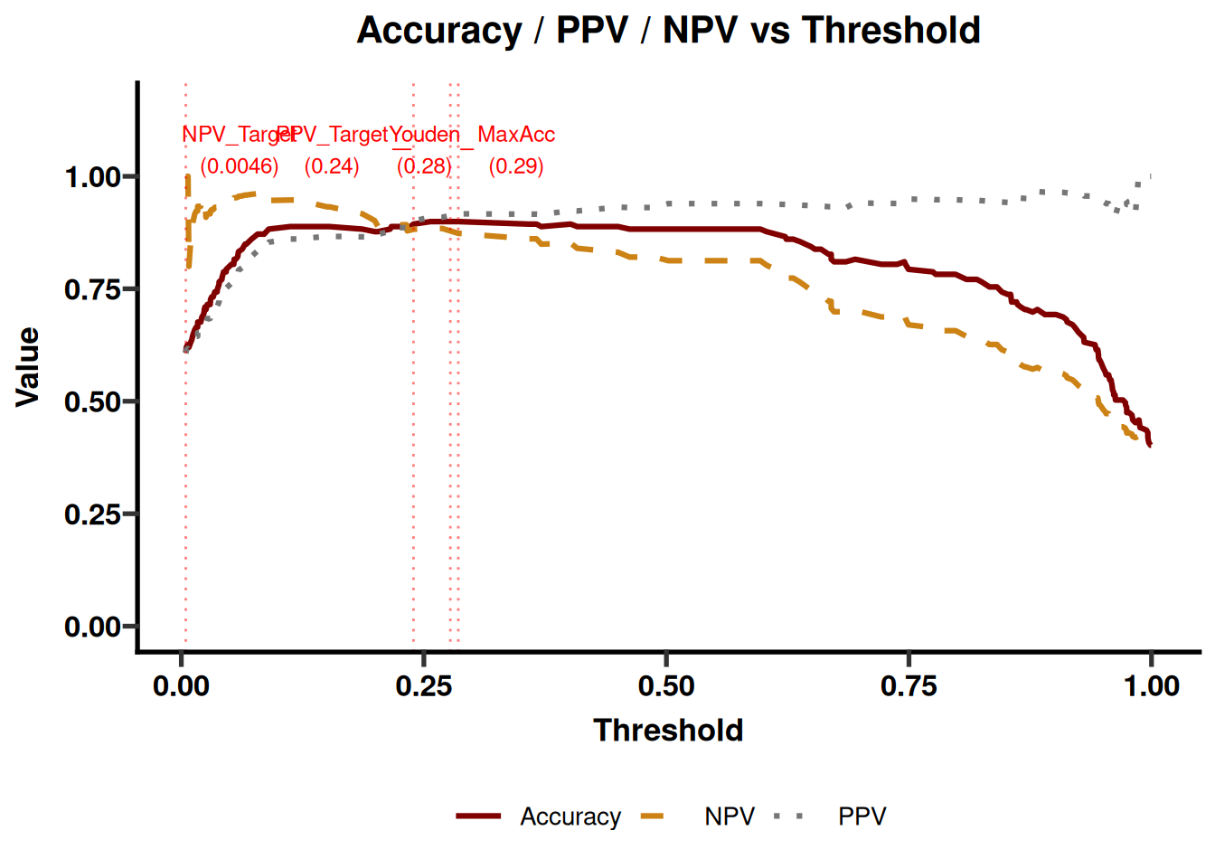
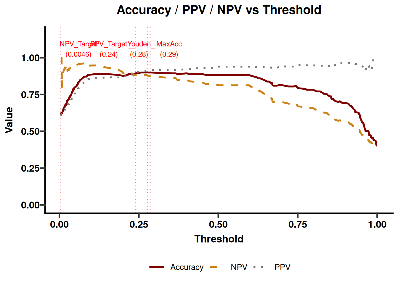
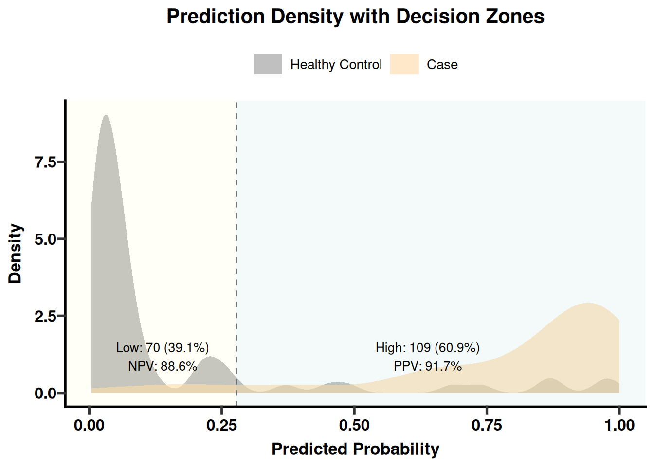
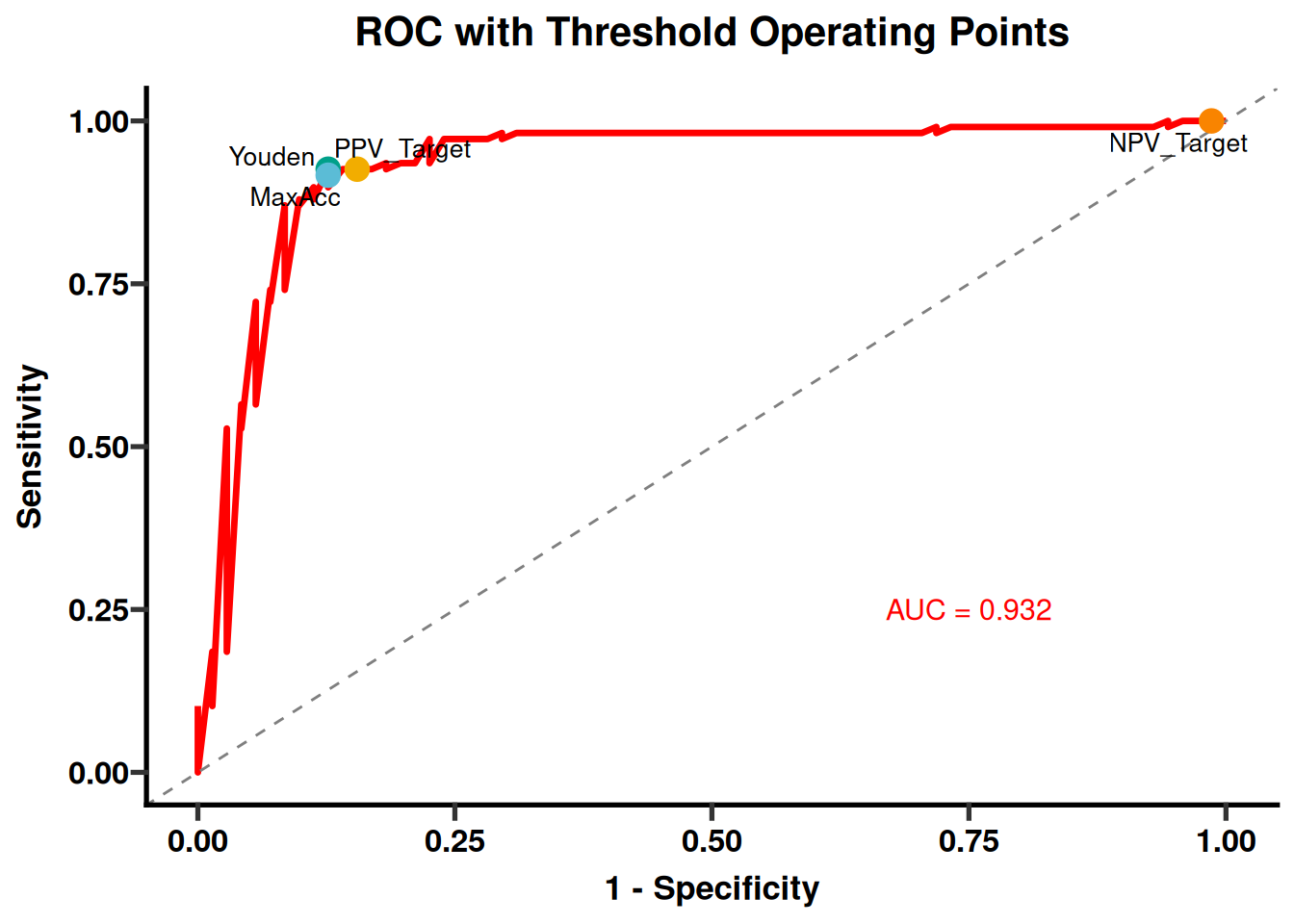
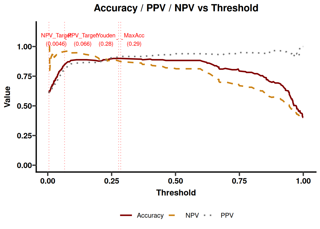
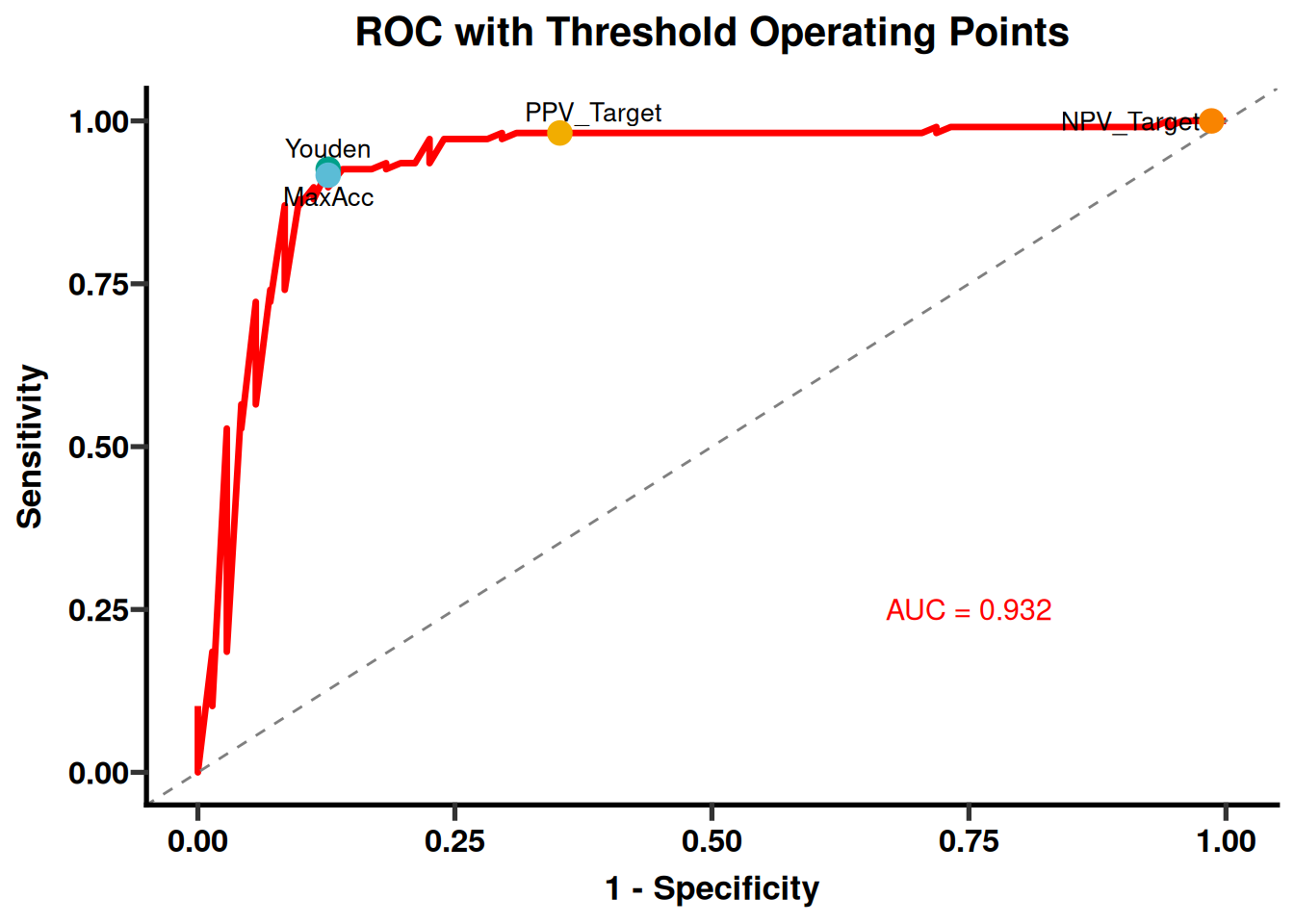
thresh <- CalculateThresholds(model_obj, target_ppv = 0.9, target_npv = 0.9, target_acc = TRUE)
names(thresh$thresholds)
ApplyThreshold(thresh, which_threshold = "Youden")
ApplyThreshold(thresh, which_threshold = "PPV_Target")
ApplyThreshold(thresh, which_threshold = "NPV_Target")
ApplyThreshold(thresh, custom_threshold = 0.5)
# From Step 2 onward, run plots in any order and adjust parameters as needed
PlotThresholdAccuracy(thresh, save_plot = TRUE, save_dir = file.path(clin_dir, "full_clinical"))
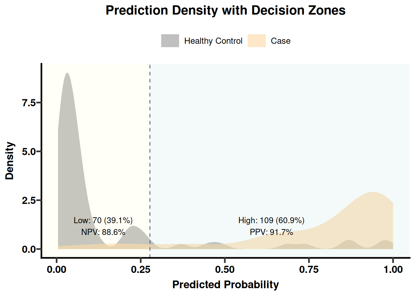
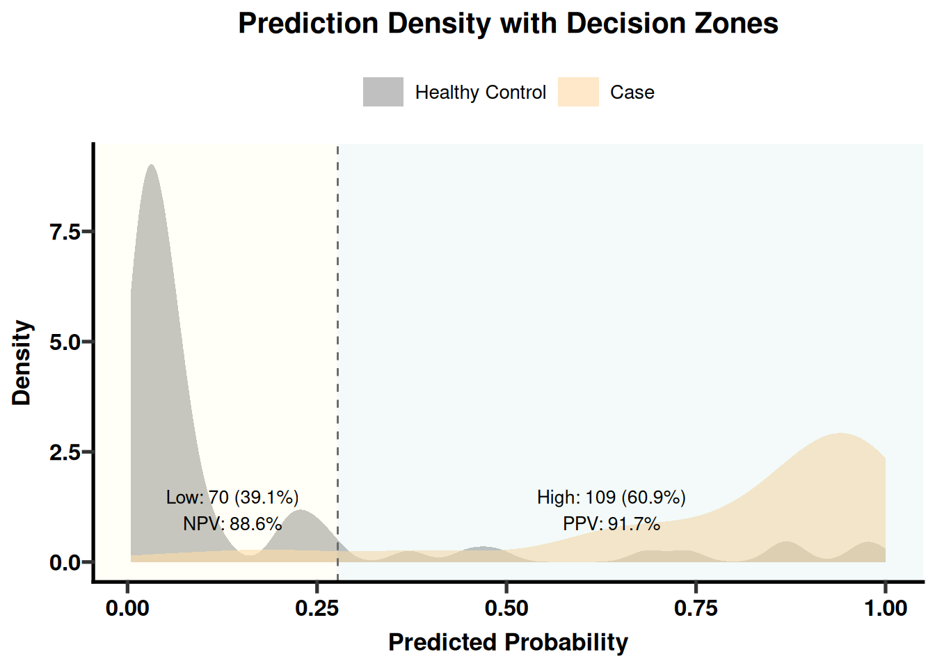
PlotThresholdDensity(thresh, save_plot = TRUE, save_dir = file.path(clin_dir, "full_clinical"))
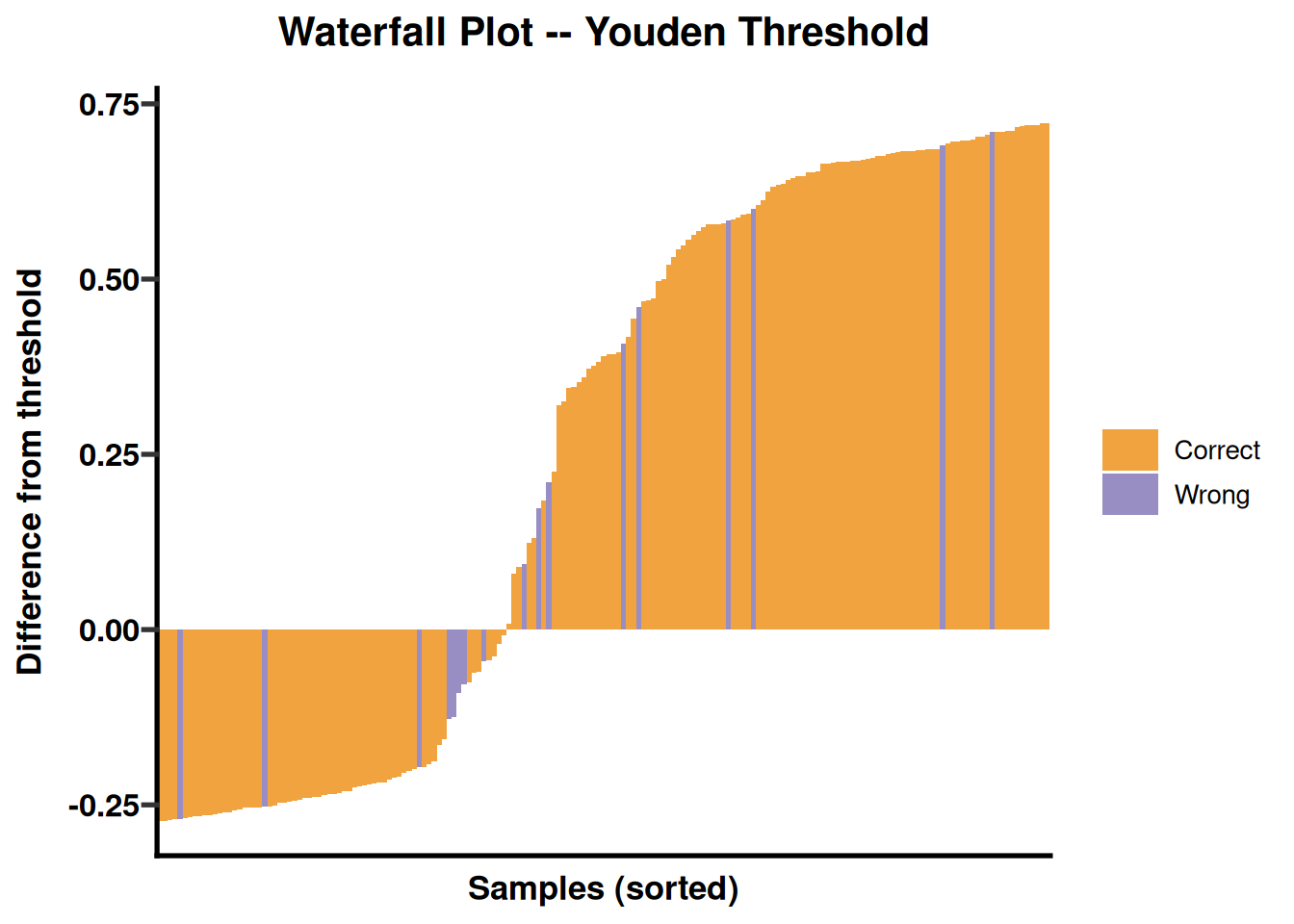
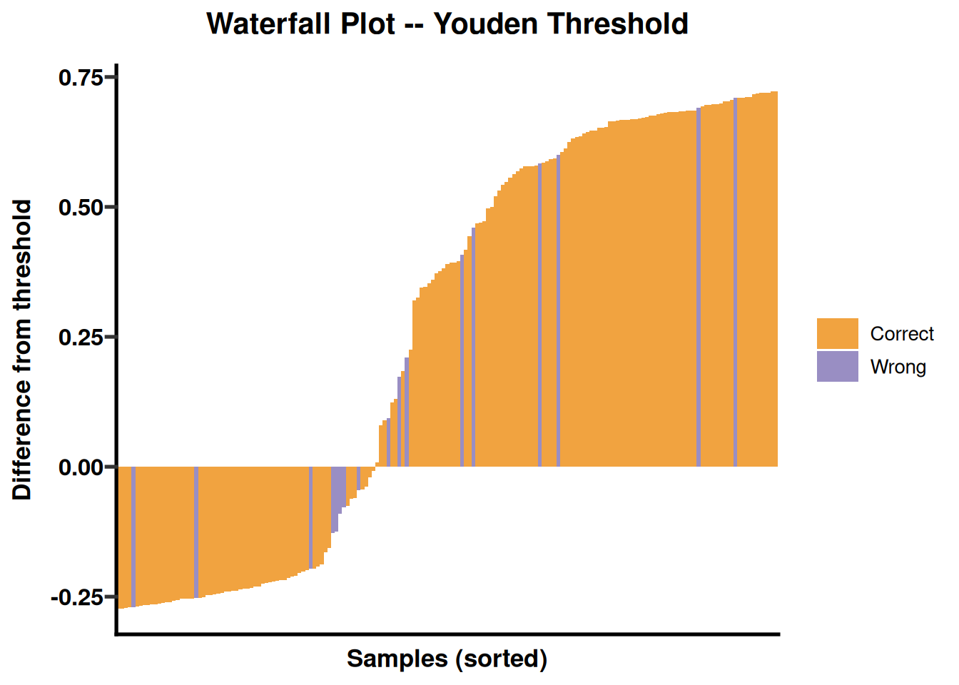
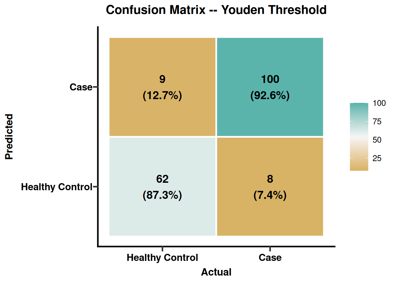
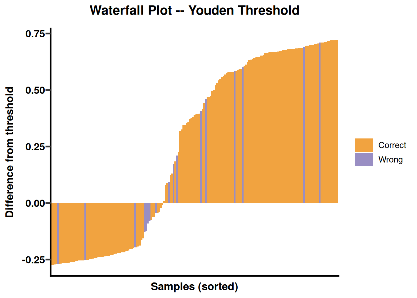
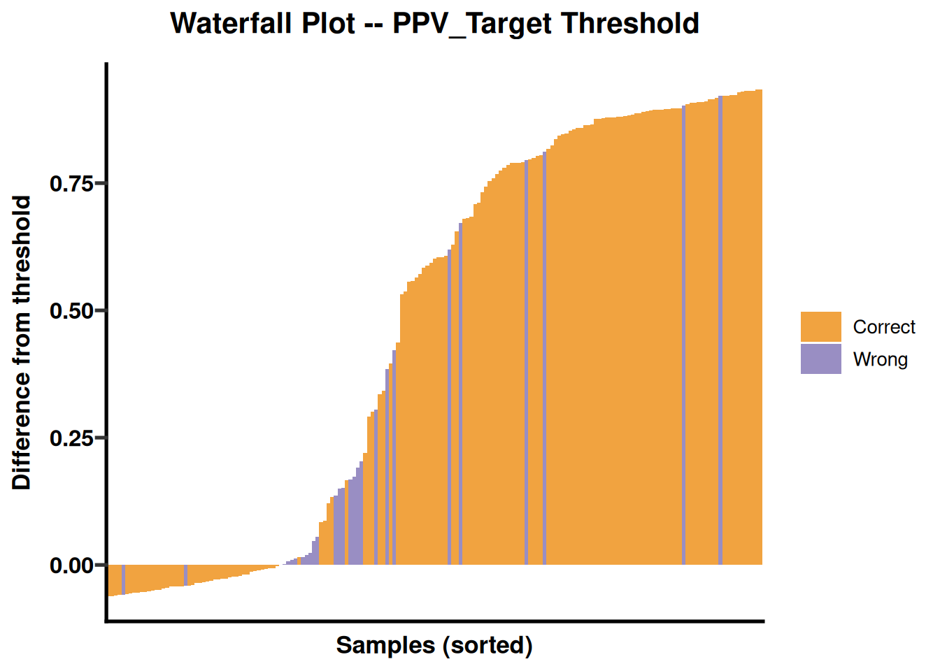
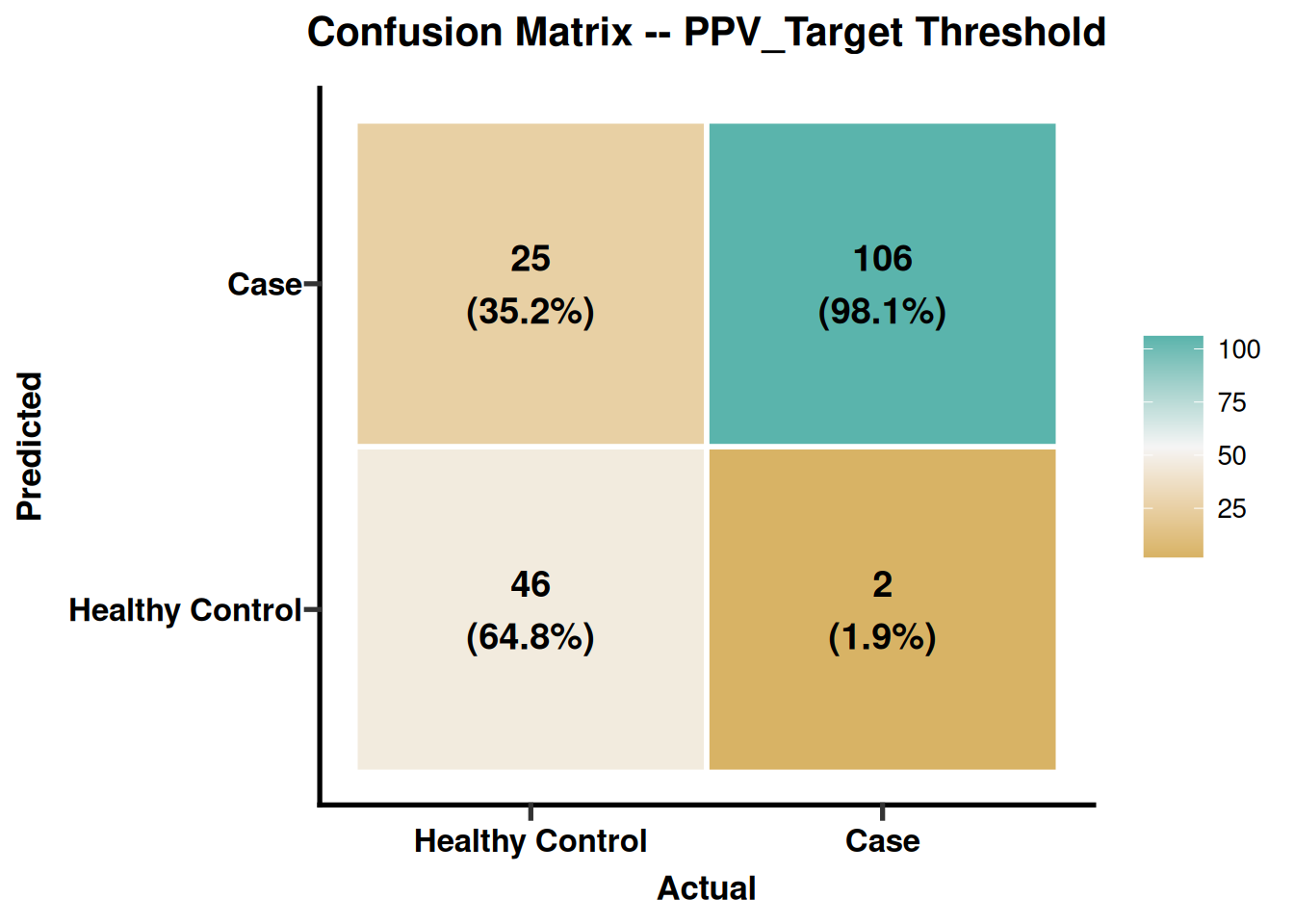
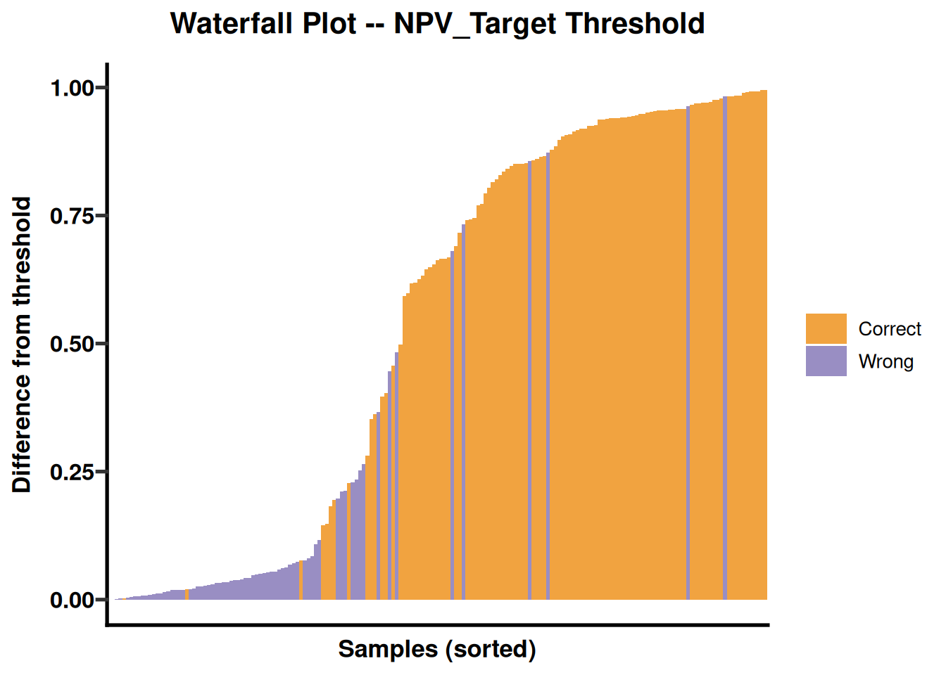
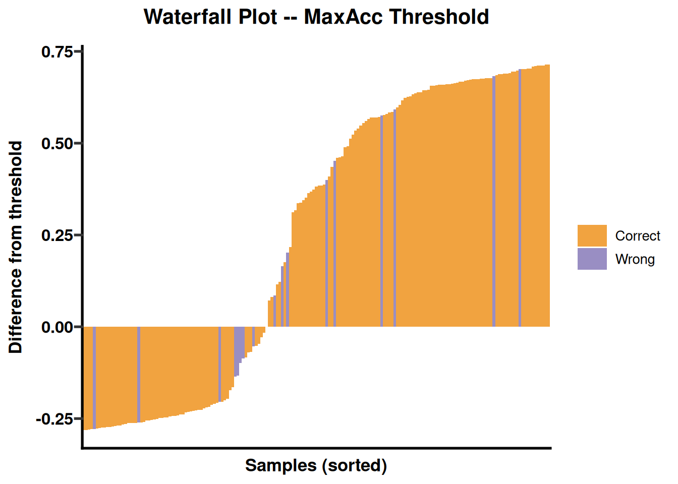
PlotThresholdWaterfall(thresh, which_threshold = "Youden", save_plot = TRUE, save_dir = file.path(clin_dir, "full_clinical"))
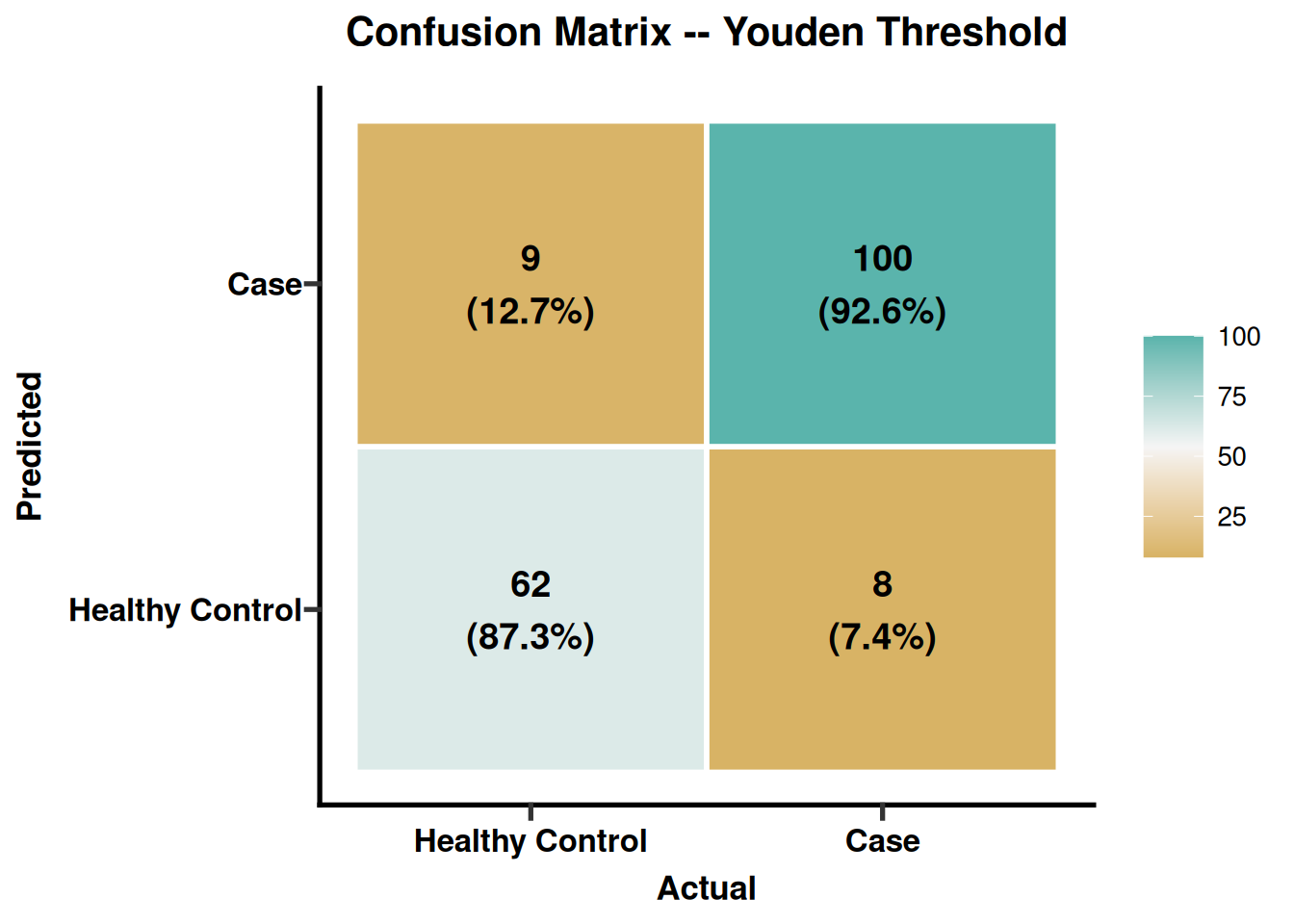
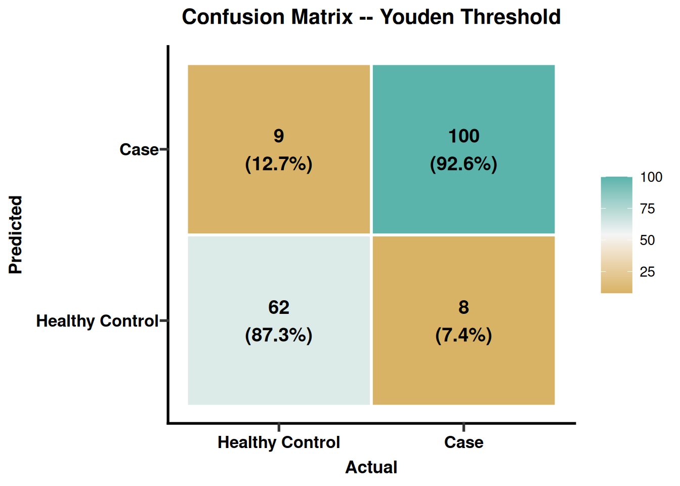
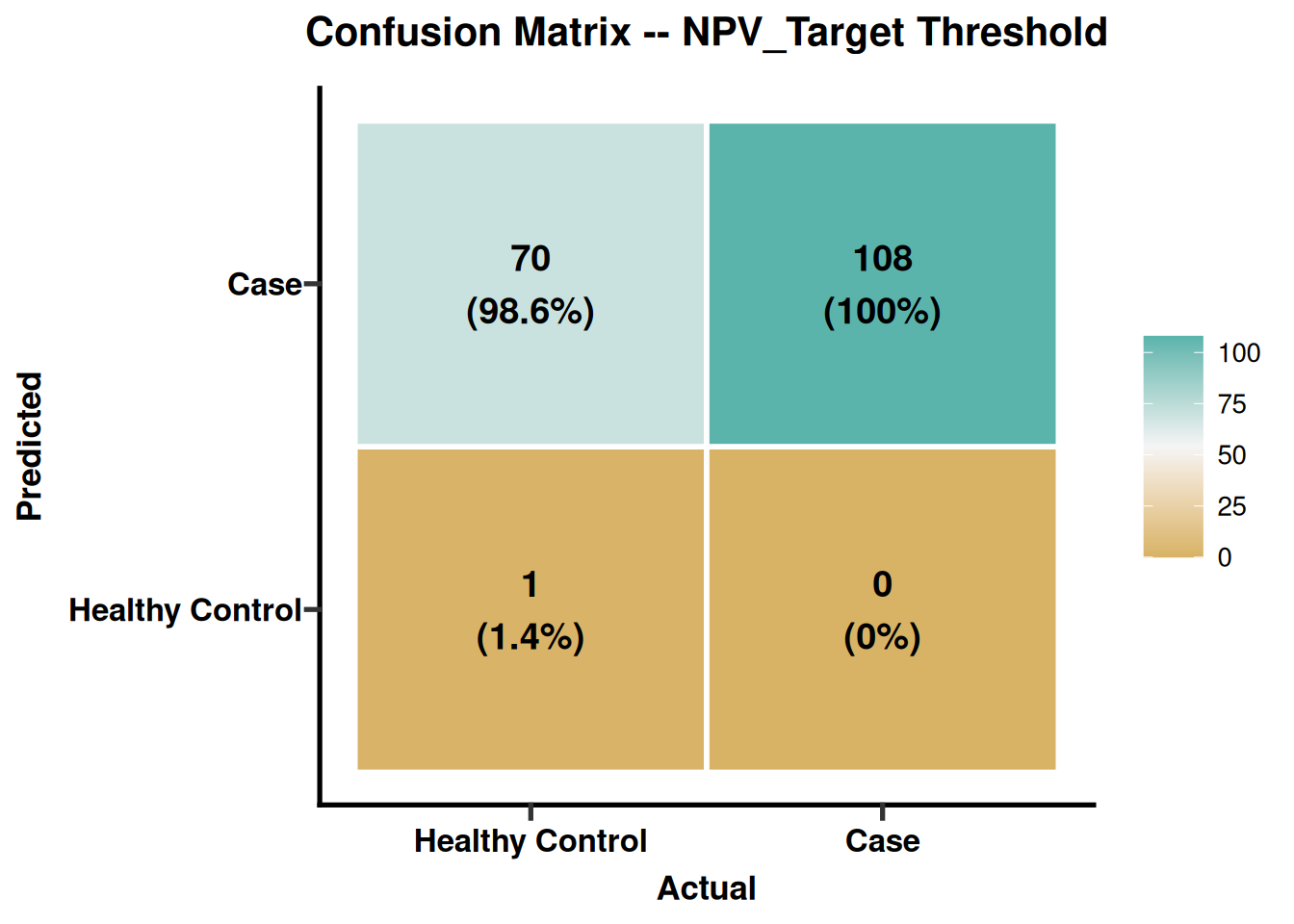
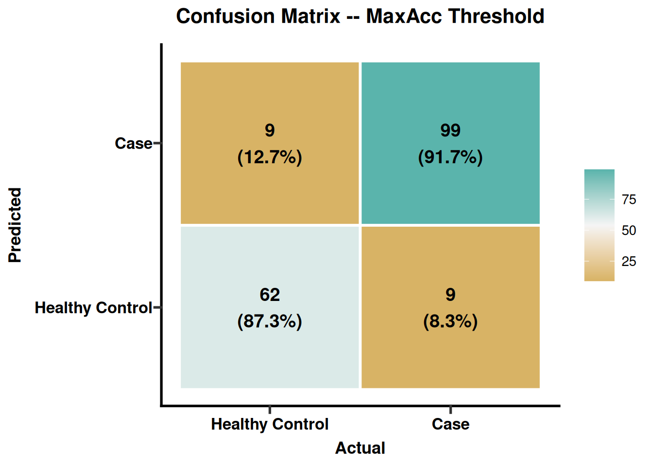
PlotThresholdConfusion(thresh, which_threshold = "Youden", save_plot = TRUE, save_dir = file.path(clin_dir, "full_clinical"))
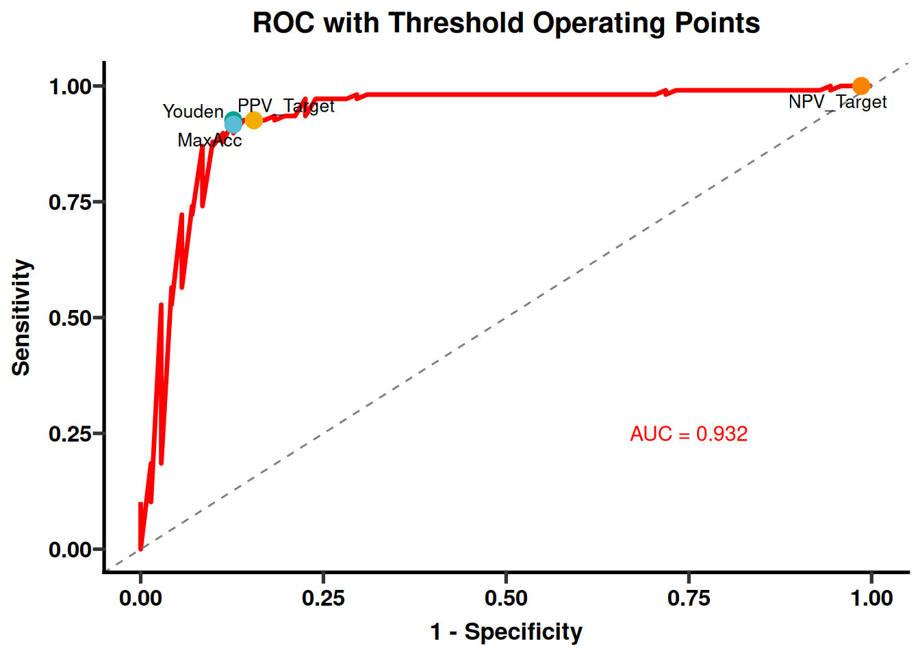
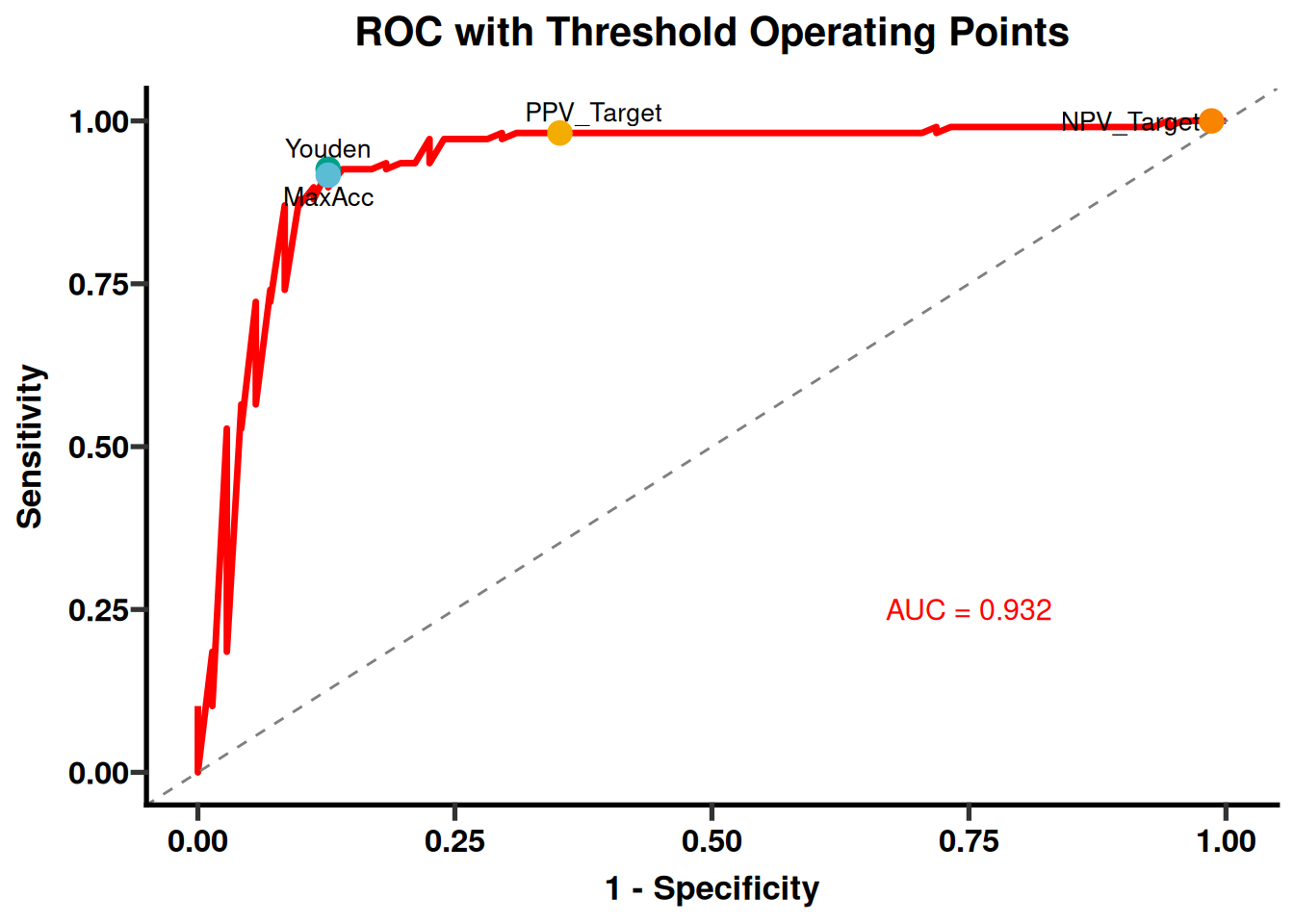
PlotThresholdROC(thresh, save_plot = TRUE, save_dir = file.path(clin_dir, "full_clinical"))
ClinicalThreshold(model_obj, target_ppv = 0.8, target_npv = 0.9,
                   save_plot = TRUE, save_dir = file.path(clin_dir, "thresholds"))
# --- 12.2 Compare against an external / simulated model ---------------------
# ---- Code with English comments ----

# The positive class is the second factor level of the outcome column.
# NOTE: do not reconstruct the probability-column name with a "X" prefix --
# that was an artifact of a 0/1-coded label ("X1"). caret names the `type =
# "prob"` columns after the factor LEVELS themselves, and make syntactically
# valid names (so "Healthy Control" becomes "Healthy.Control"). With the
# readable labels used since icare 1.1 the positive level is, e.g., "Case",
# and the matching probability column is named identically.
positive <- levels(factor(test_data[[model_obj@group_col]]))[2]

# Calculate classification thresholds (e.g., probability cutoffs) from the internal model
# to achieve target Positive Predictive Value (PPV) = 0.8, Negative Predictive Value (NPV) = 0.9,
# and also optimize for accuracy (target_acc = TRUE).
thresh_internal <- CalculateThresholds(model_obj, target_ppv = 0.8, target_npv = 0.9, target_acc = TRUE)

# Set seed for reproducibility of the random perturbation step.
set.seed(456)

# Obtain predicted probabilities for the positive class from the internal random forest model
# applied to the test data.
my_probs <- predict(model_obj@train.models$rf, test_data, type = "prob")[, positive]

# Simulate predictions from an "external" model by adding random noise to the logit of the probabilities.
# This is a crude way to generate a second set of probability estimates for comparison.
# - Add a small constant (1e-6) to avoid log(0) issues.
# - Transform to logit scale, add Gaussian noise (sd = 0.5), then back-transform to probability scale.
rdoc_probs <- plogis(qlogis(my_probs + 1e-6) + rnorm(length(my_probs), mean = 0, sd = 0.5))
# Ensure probabilities remain within [0,1] after perturbation.
rdoc_probs <- pmax(0, pmin(1, rdoc_probs))

# Calculate thresholds from the simulated external model's probabilities,
# using the same performance targets (PPV, NPV, accuracy).
# Note: `positive` is the level derived above, not a hardcoded "1" -- the
# outcome factor carries readable labels since icare 1.1, and
# CalculateThresholdsFromProbs() checks it against levels(true).
thresh_external <- CalculateThresholdsFromProbs(
  probs = rdoc_probs, true = factor(test_data[[model_obj@group_col]]),
  positive = positive, target_ppv = 0.8, target_npv = 0.9, target_acc = TRUE
)

# Compare the two sets of thresholds by plotting performance metrics (e.g., confusion matrices)
# for the internal model ("Your Model") vs. the external simulation ("External Model").
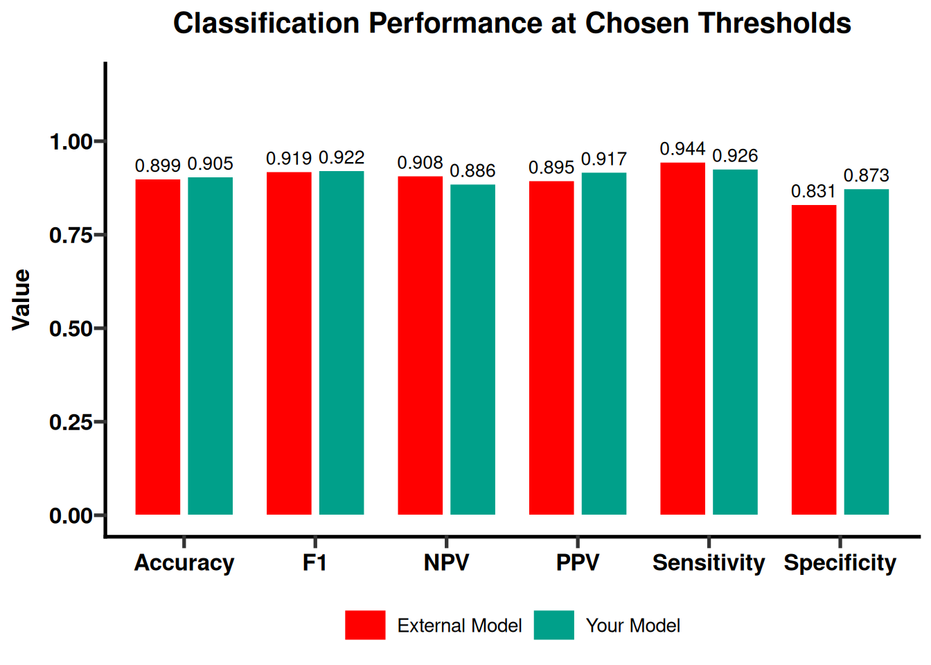
CompareClassification(thresh_internal, thresh_external,
                      label1 = "Your Model", label2 = "External Model",
                      save_plot = TRUE, save_dir = file.path(clin_dir, "comparison"))
# Plot ROC curves with the identified thresholds overlaid, comparing both models.
# The internal thresholds are used as the primary set; the external model is added for comparison.
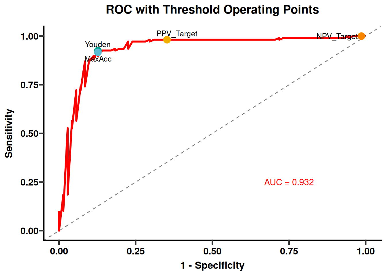
PlotThresholdROC(thresh_internal, compare_model = thresh_external,
                 compare_label = "External Model",
                 save_plot = TRUE, save_dir = file.path(clin_dir, "comparison"))

# --- 12.3 Reclassification: NRI / IDI between two models --------------------
nri_dir <- sub_dir("06_nri_idi")
true_labels <- factor(test_data[[model_obj@group_col]])
ref_prob <- predict(model_obj@train.models$rf,  test_data, type = "prob")[, positive]
new_prob <- predict(model_obj@train.models$svmRadial, test_data, type = "prob")[, positive]

# Scenario A: both models judged against the same clinical risk thresholds.
# Set directories: keep these figures inside the chapter's output tree
# (nri_dir was created above) instead of the working directory.
save_dir <- file.path(nri_dir, "manual_results")
dir.create(save_dir, recursive = TRUE, showWarnings = FALSE)

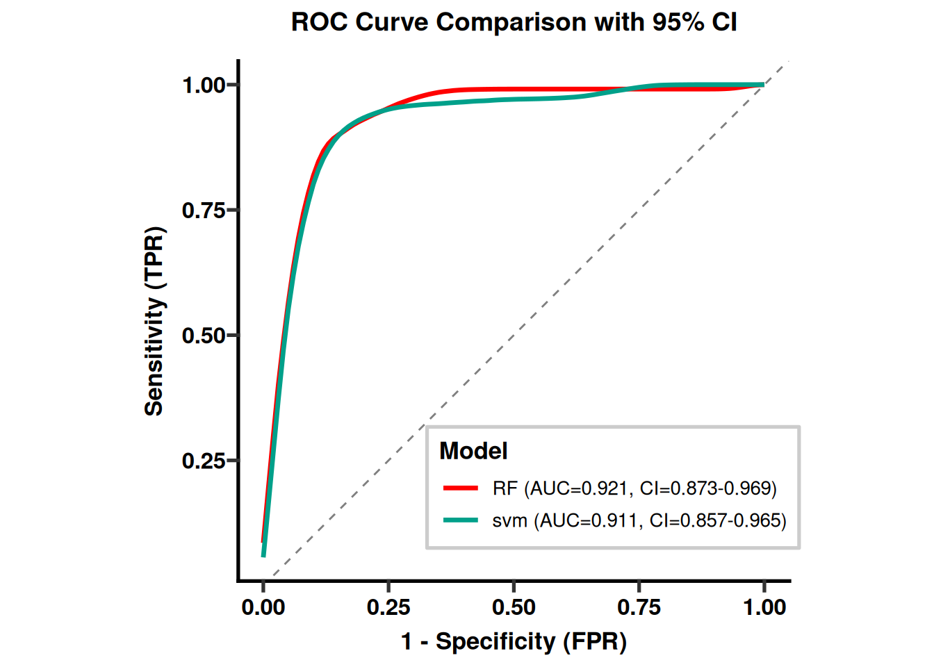
# ROC
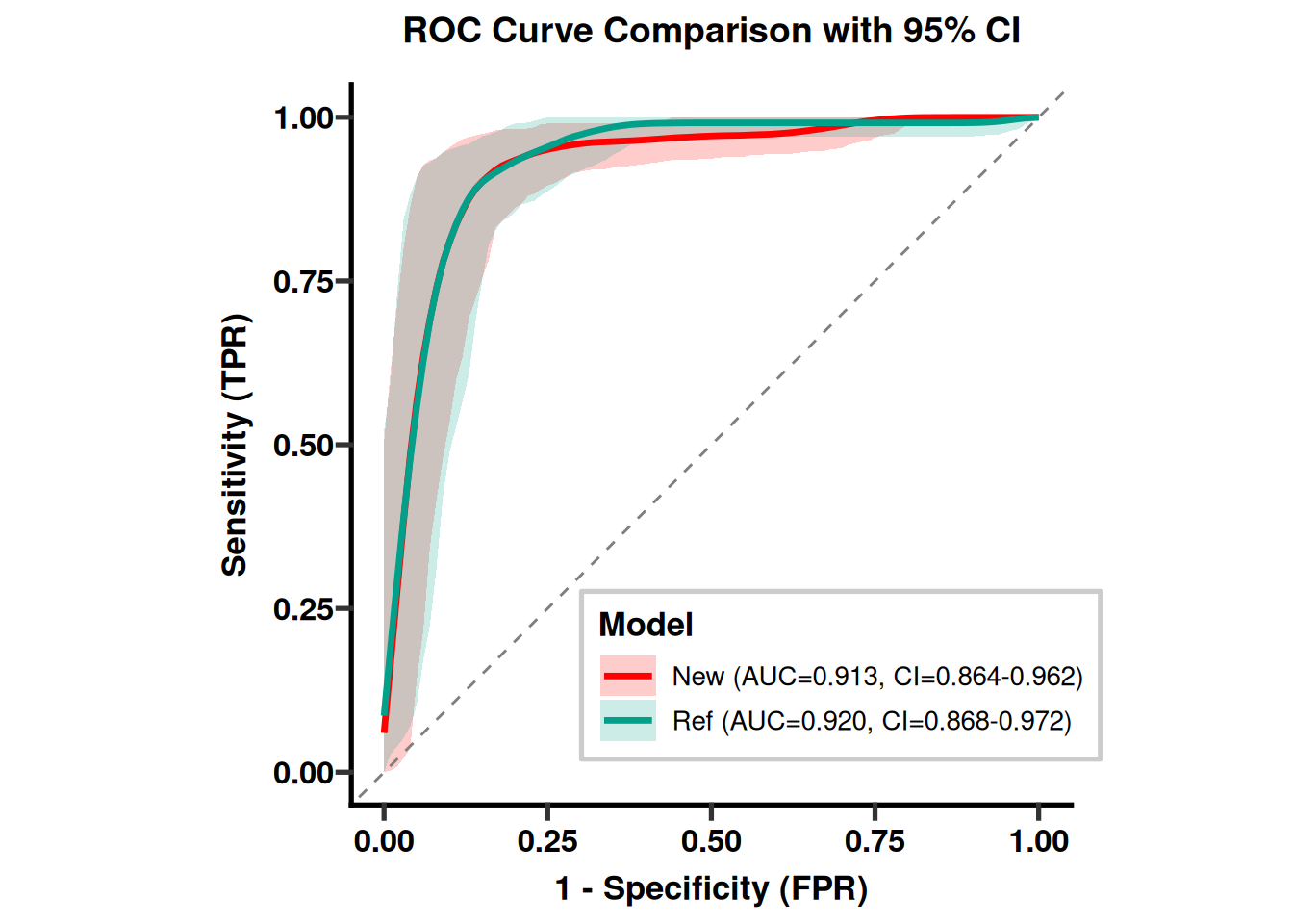
PlotROCCompare(true_labels, ref_prob, new_prob,
               labels = c("Ref", "New"), save_plot = TRUE, save_dir = save_dir)
# IDI
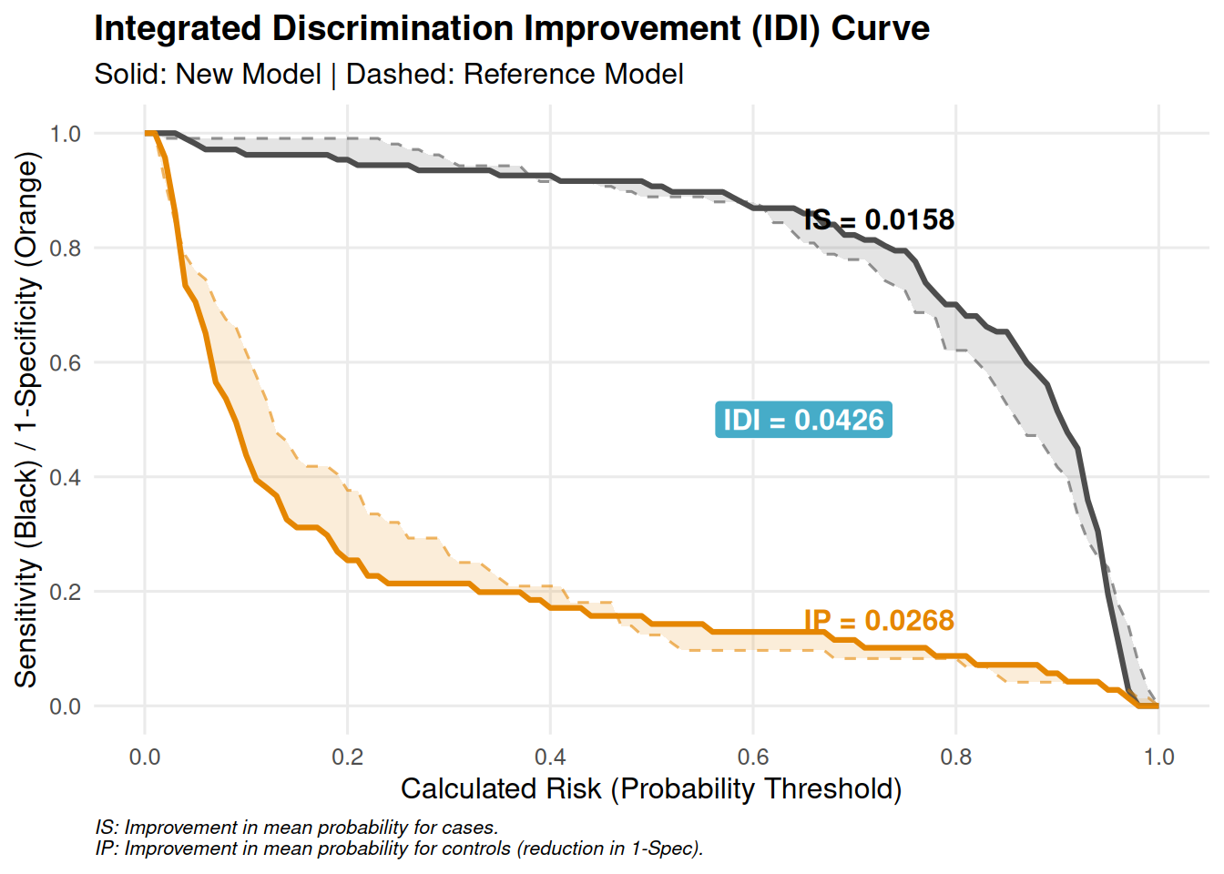
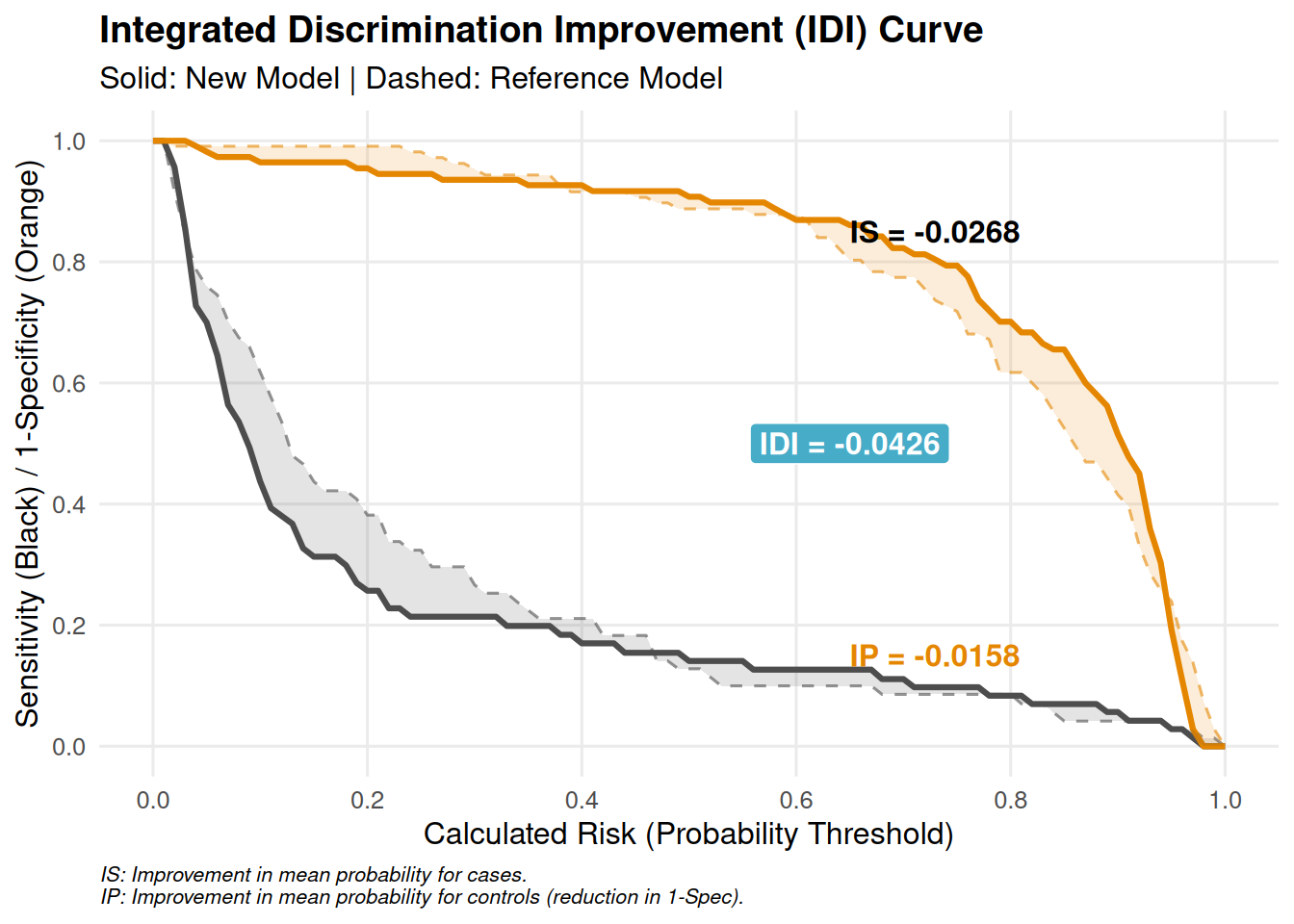
idi <- PlotIDICurve(true_labels, ref_prob, new_prob, positive = positive,
                    save_plot = TRUE, save_dir = save_dir)
idi
# NRI calculation
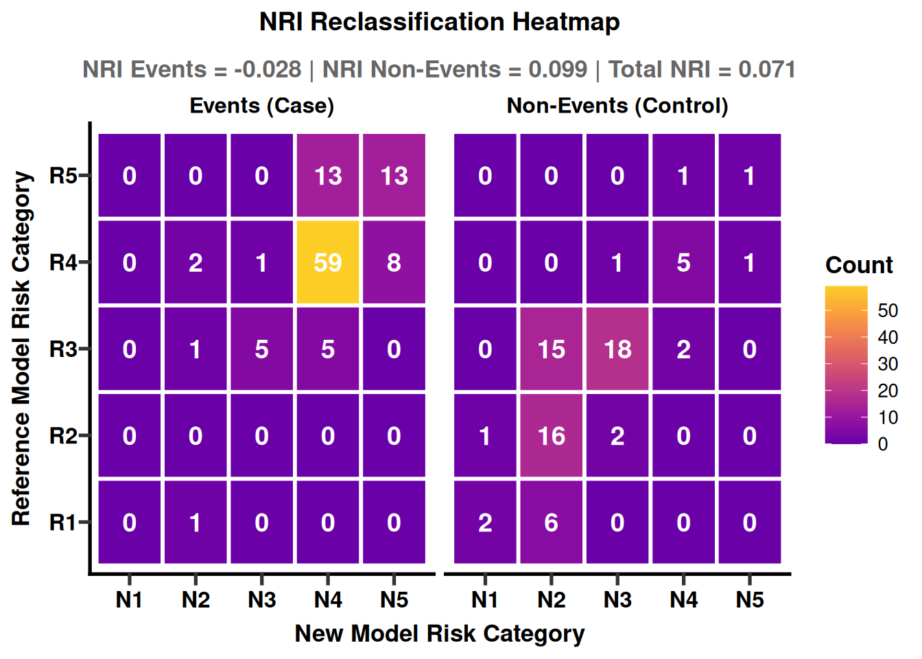
nri <- CalculateCategoryNRI(true_labels, ref_prob, new_prob,
                            risk_thresholds = c(0.02, 0.1, 0.5, 0.95))
# Export numeric results
cat("\nNRI Events:", nri$nri_events,
    "\nNRI Non-Events:", nri$nri_nonevents,
    "\nTotal NRI:", nri$nri_total, "\n")
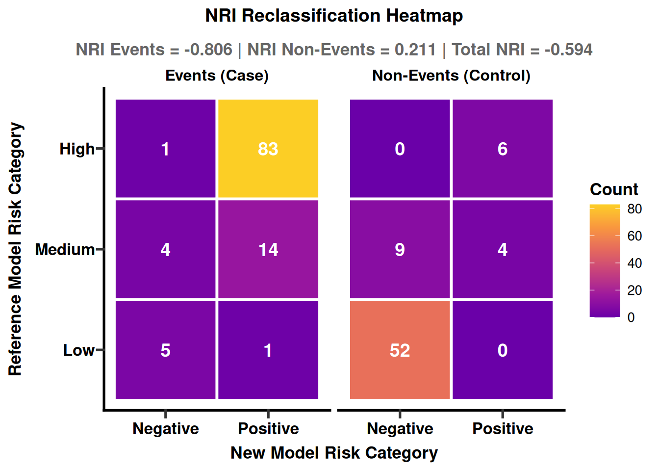
# NRI heatmap
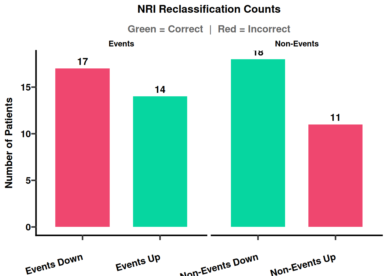
PlotNRIHeatmap(nri, save_plot = TRUE, save_dir = save_dir)
# NRI bar plot
PlotNRIBars(nri, save_plot = TRUE, save_dir = save_dir)
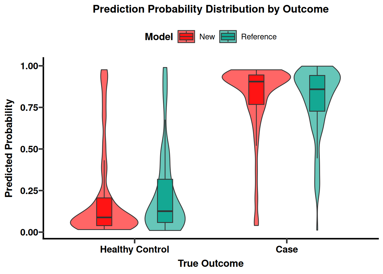
# Probability distributions
# outcome_labels must be given in the order of levels(true_labels); passing
# c("0","1") here would relabel the readable classes back to meaningless codes.
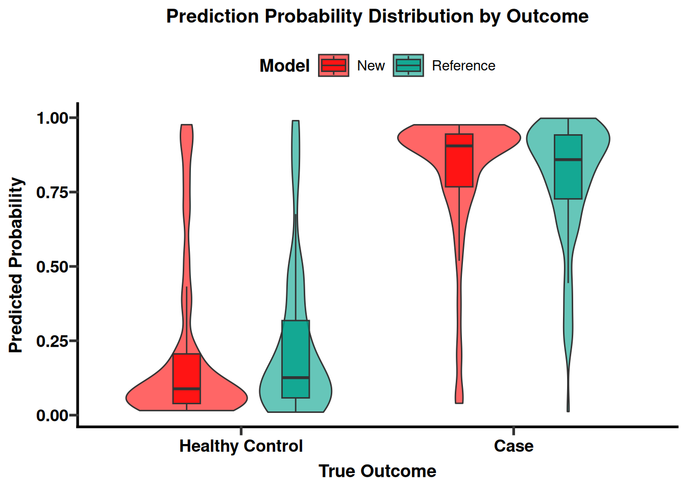
PlotPredDist(true_labels, ref_prob, new_prob,
             labels = c("Ref", "New"), outcome_labels = levels(true_labels),
             save_plot = TRUE, save_dir = save_dir)
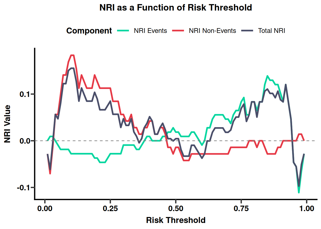
# Threshold–NRI curve (optional)
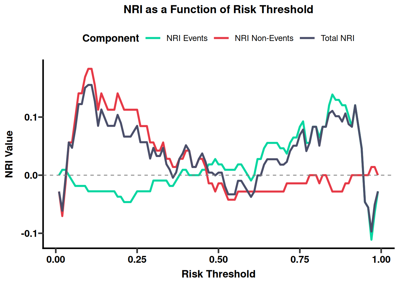
PlotThresholdNRI(true_labels, ref_prob, new_prob,
                 save_plot = TRUE, save_dir = save_dir)
# Scenario B: models compared using their own, independent thresholds.
if(F){
NRI_IDI_Analysis(
  ref_prob = ref_prob, new_prob = new_prob, truth = true_labels,
  ref_thresholds = c(0.02, 0.1, 0.5, 0.95), new_thresholds = c(0.05, 0.4),
  ref_category_labels = c("I", "II", "III", "IV", "V"),
  new_category_labels = c("Low", "Intermediate", "High"),
  labels = c("Reference RF", "New Model"), outcome_labels = c("Benign", "Malignant"),
  show_ci = FALSE, save_dir = file.path(nri_dir, "independent_thresholds"))
}

# Scenario C: individual building blocks, for full control over each plot.
nri_res <- CalculateCategoryNRI(true_labels, ref_prob, new_prob,
                                 ref_thresholds = c(0.3, 0.7), new_thresholds = c(0.5))
print(nri_res$nri_total)
PlotNRIHeatmap(nri_res, ref_category_labels = c("Low", "Medium", "High"),
               new_category_labels = c("Negative", "Positive"),
               save_plot = TRUE, save_dir = file.path(nri_dir, "heatmap"))
PlotIDICurve(true_labels, ref_prob, new_prob, risk_thresholds = c(0.02, 0.1, 0.5, 0.95),
             save_plot = TRUE, save_dir = file.path(nri_dir, "idi"))
PlotROCCompare(true_labels, ref_prob, new_prob, labels = c("RF", "svm"), show_ci = FALSE,
               save_plot = TRUE, save_dir = file.path(nri_dir, "roc"))
PlotPredDist(true_labels, ref_prob, new_prob, labels = c("RF", "New"),
             outcome_labels = levels(true_labels), save_plot = TRUE, save_dir = file.path(nri_dir, "dist"))
PlotThresholdNRI(true_labels, ref_prob, new_prob, save_plot = TRUE,
                  save_dir = file.path(nri_dir, "threshold_scan"))
# =============================================================================
````
### 13 Deployment
This section applies the trained object to new samples. Validate input format, performance, and target population in an independent cohort before deployment.
````{r}
#| label: module2-advanced-25
#| cache: false
#| echo: true
#| message: false
#| warning: false
#| fig-show: hold
#| out-width: '100%'
# 13. Deployment
# =============================================================================
# Collect all ensemble objects in a named list
model_obj@process.info$ensembles <- list(
  "Stacking"        = model_stack,
  "Average"         = model_avg,
  "Weighted"        = model_wgt,
  "CustomWeighted"  = model_custom
)

# Validate saved objects
names(model_obj@process.info$ensembles)
# Wrap the trained model(s), the preprocessing recipe, and readable class
# labels into a single deployment object that can be used programmatically
# or through the bundled Shiny app.
deploy_manager <- icare::ModelDeployment(
  object            = model_obj,
  preproc           = preProc,
  class_labels      = c("NEGATIVE", "POSITIVE"),
  model_description = "Ensemble platform for clinical outcome prediction."
)

demo_records <- head(model_obj@clean.df, 20)

## 13.1 High-sensitivity screening mode (lower threshold, e.g. for triage).
screen_res<-deploy_manager$predict_fn(demo_records, selected_model = "Ensemble Stacking")
pos_probs <- screen_res[, 2]
screen_diag <- ifelse(pos_probs >= 0.3, "POSITIVE", "NEGATIVE")
screen_diag
## 13.2 Compare two specific algorithms at a standard threshold.
res_rf   <- deploy_manager$predict_fn(demo_records, selected_model =  "rf")
res_svm  <- deploy_manager$predict_fn(demo_records, selected_model ="svmRadial")
diag_rf  <- ifelse(res_rf[, 2]  >= 0.5, "POSITIVE", "NEGATIVE")
diag_svm <- ifelse(res_svm[, 2] >= 0.5, "POSITIVE", "NEGATIVE")

## 13.3 Interactive Shiny app — only launched in an interactive session so
## this script can still run non-interactively (e.g. via `Rscript`).
library(bslib); library(shiny); library(plotly)
if (interactive()) {
  icare::deploy_clinlab_app(deploy_manager, title = "Clinlabomics Intelligence")
} else {
  message("Interactive deployment app skipped during non-interactive book rendering.")
}


# =============================================================================
````
### 14 Save the Final Model Object
This section trains and compares candidate models. Select models using discrimination, calibration, stability, and clinical utility together.
````{r}
#| label: module2-advanced-26
#| echo: true
#| message: false
#| warning: false
#| fig-show: hold
#| out-width: '100%'
# 14. Save the Final Model Object
# =============================================================================
saveRDS(model_obj, file = "model_obj.rds")

cat("\n========================================\n")
cat("Module 2 (advanced) pipeline finished successfully!\n")
cat("All figures/tables saved under:", OUTPUT_DIR, "\n")
cat("========================================\n")
````