# Module 3: Unsupervised Subtyping — Advanced
The advanced `Subtyping` workflow normalizes independent development and validation sets, compares K-means, latent profile analysis (LPA), and NMF, and evaluates t-SNE/UMAP structure, internal cluster quality, cross-method agreement, marker profiles, silhouettes, alluvial relationships, and deployment to new samples.
## Preventing Information Leakage
Split the data first, fit min–max parameters on the development set, and apply them unchanged to validation data. The workflow also checks numeric types and removes zero-variance features. Embeddings are exploratory: choose and validate a subtype solution using stability, agreement, marker reproducibility, and clinical usefulness rather than visual separation alone.
## Step-by-step Workflow
The workflow is divided into short stages. Each note explains the purpose, key checks, and interpretation limits. Generated plots and tables appear directly below their code chunk.
### About this chapter
**Audience.** Advanced users who want to compare multiple clustering methods, validate them, and produce publication-style figures.
**Input.** Requires `stat_obj.rds`, produced by Module 1.
The chapter runs end to end as one session:
1. **CONFIG**
2. **Load Data and Convert to a Subtyping Object**
3. **Split into Train / Validation Sets, then Normalize**
4. **Clustering — Three Complementary Methods**
- **Estimate the best rank (= number of subtypes) across a candidate range.**
- **Pick the best rank from the estimation above.**
- **Assign each training sample to a subtype.**
- **Refit with more NMF runs and save a re-usable model object, so new**
5. **Predict Subtypes on the Validation Split**
6. **Dimensionality Reduction for Visualization (t-SNE & UMAP)**
7. **Clustering Quality Evaluation**
8. **Consistency Between the Three Clustering Methods**
9. **Subtype-Specific Marker Features & Enhanced Visualization**
10. **Deployment: Predict Subtypes for New Samples**
11. **Save Final Objects**
### 0 CONFIG
This section defines seeds, output paths, and dependencies. Update these paths and key parameters first when using new data.
````{r}
#| label: module3-advanced-09
#| echo: true
#| message: false
#| warning: false
#| fig-show: hold
#| out-width: '100%'
# 0. CONFIG
# ---------------------------------------------------------------------------
rm(list = ls())
library(icare)

INPUT_STAT_OBJ  <- "stat_obj.rds"
OUTPUT_DIR      <- "./Module3_Advanced_Output"
GROUP_COL       <- "group"   # the outcome/group column carried over from Module 1
SEED            <- 123

dir.create(OUTPUT_DIR, showWarnings = FALSE, recursive = TRUE)
# Register OUTPUT_DIR with the package rather than defining a local sub_dir().
# icare already ships sub_dir(); a local definition shadows it only inside this
# script, so functions INSIDE the package that call sub_dir() themselves would
# still resolve it in the icare namespace and write somewhere else. Calling
# set_output_root() points both this script and the package at the same tree.
set_output_root(OUTPUT_DIR)

# =============================================================================
````
### 1 Load Data and Convert to a Subtyping Object
This section imports and organizes the data. Check dimensions and variable coding before continuing.
````{r}
#| label: module3-advanced-10
#| echo: true
#| message: false
#| warning: false
#| fig-show: hold
#| out-width: '100%'
# 1. Load Data and Convert to a Subtyping Object
# =============================================================================
stat_obj <- readRDS(INPUT_STAT_OBJ)
InspectObject(stat_obj)
sub_obj <- ConvertObject(stat_obj, to = "Subtyping")
InspectObject(sub_obj)
features=colnames(sub_obj@clean.data)[colnames(sub_obj@clean.data)!='sex']
sub_obj@clean.data <- sub_obj@clean.data[, features, drop = FALSE]
# =============================================================================
````
### 2 Split into Train / Validation Sets, then Normalize
This section preprocesses the data. Review missingness, outlier handling, and normalization before accepting the defaults.
````{r}
#| label: module3-advanced-12
#| echo: true
#| message: false
#| warning: false
#| fig-show: hold
#| out-width: '100%'
# 2. Split into Train / Validation Sets, then Normalize
# =============================================================================
# IMPORTANT: split BEFORE fitting any normalization parameters — mirrors the
# pattern used in Module 2 (createDataPartition first, then preProcess() fit
# on the training split only, never on the full dataset). Fitting min-max
# parameters on the full data (train+validation combined) and only THEN
# splitting would let validation-set values leak into the scaling applied to
# the validation set itself — the opposite of what we want.
set.seed(SEED)
split <- SplitSubtypingObject(sub_obj, p = 0.7, stratify_by = GROUP_COL)
# min-max scaling keeps all features non-negative, which NMF requires.
# Fit normalization on the TRAINING split only.
# IMPORTANT: pass group_col = GROUP_COL explicitly. Sub_normalize_process()'s
# default is the literal string "group", so renaming GROUP_COL in the CONFIG
# block and leaving this call alone would normalize against the wrong name.
# Since the 1.1 label contract the outcome lives in info.data and never in
# clean.data, so it can no longer leak into scale.data; the defensive check
# below still guards the assumption that matters -- every column handed to
# K-means / LPA / NMF must be numeric.
sub_train <- Sub_normalize_process(split$train, normalize_method = "min_max",
                                   group_col = GROUP_COL)
cat("Normalization completed. scale.data dimensions:", dim(sub_train@scale.data), "\n")
# Defensive check: confirm every remaining column really is numeric before
# it reaches K-means/LPA/NMF, all three of which require a purely numeric
# input matrix.
non_numeric_cols <- names(sub_train@scale.data)[!vapply(sub_train@scale.data, is.numeric, logical(1))]
if (length(non_numeric_cols) > 0) {
  stop("Non-numeric column(s) in scale.data: ", paste(non_numeric_cols, collapse = ", "),
       ". Check group_col above, or drop these columns from clean.data first.")
}

# Extract the normalization parameters learned on the TRAINING split only, so
# they can be re-applied identically to the validation split without letting
# validation-set information leak into its own scaling (avoids data leakage,
# analogous to Module 2's preProcess() being fit on split.data$training only).
norm_params <- Sub_extract_norm_params(sub_train, verbose = TRUE)
# Apply the training-derived parameters to the validation split — the
# validation set never contributes to its own normalization statistics.
sub_test <- Sub_apply_norm_params(split$test, norm_params = norm_params, verbose = TRUE)
cat("Train set:", nrow(sub_train@clean.data), "samples | Validation set:",
    nrow(sub_test@clean.data), "samples\n")
# Remove zero-variance columns — otherwise K-means' internal PCA step errors out.
sub_train@scale.data <- remove_constant_columns(sub_train@scale.data)
sub_train@clean.data <- sub_train@clean.data[, colnames(sub_train@scale.data), drop = FALSE]

# Keep the validation split's feature set aligned with the (possibly reduced)
# training feature set after zero-variance removal.
common_feats <- intersect(colnames(sub_train@scale.data), colnames(sub_test@scale.data))
sub_test@scale.data <- sub_test@scale.data[, common_feats, drop = FALSE]
sub_test@clean.data <- sub_test@clean.data[, common_feats, drop = FALSE]

# =============================================================================
````
### 3 Clustering — Three Complementary Methods
This section performs the core analysis for this stage. Review the output immediately below the code and confirm that data ranges, assumptions, and results match the study design.
````{r}
#| label: module3-advanced-13
#| echo: true
#| message: false
#| warning: false
#| fig-show: hold
#| out-width: '100%'
# 3. Clustering — Three Complementary Methods
# =============================================================================
## 3.1 K-means, with the number of clusters chosen automatically (k up to 8).
cat("\n=== K-means Clustering ===\n")
sub_train <- Sub_kmeans_with_optimal_k(
  sub_train, use_scaled_data = TRUE, k.max = 8, palette_name = "Zissou1",
  save_plots = TRUE, save_dir = sub_dir("01_kmeans"), seed = SEED
)
print(table(sub_train@info.data$cluster_kmeans))
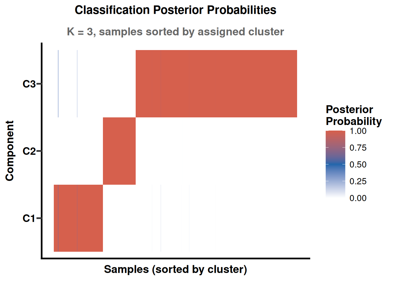
## 3.2 LPA (Latent Profile Analysis / Gaussian mixture) — a model-based
## alternative to K-means that allows clusters of different shapes/sizes.
cat("\n=== LPA Clustering ===\n")
library(mclust)
sub_train <- Sub_lpa_with_optimal_k(
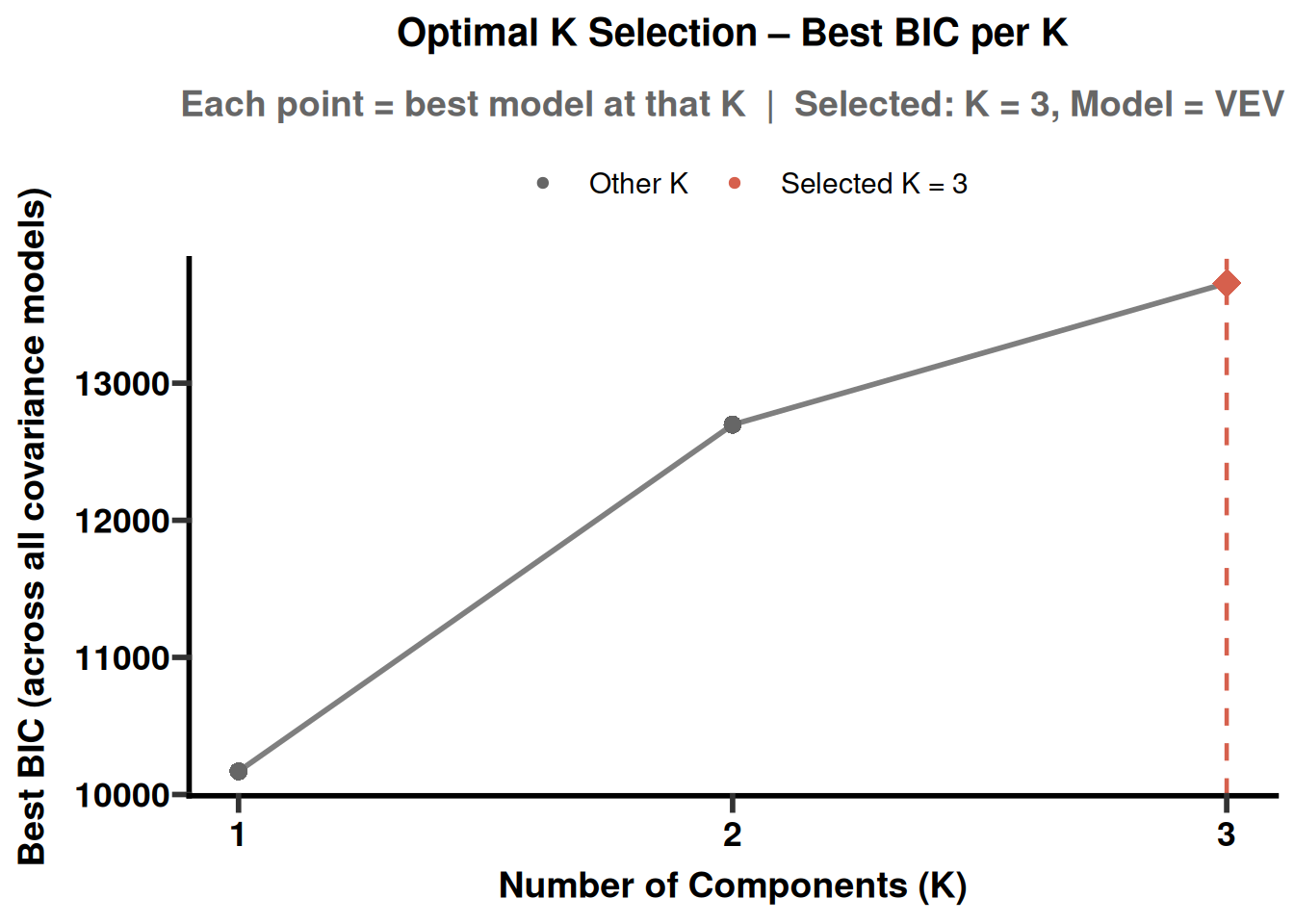
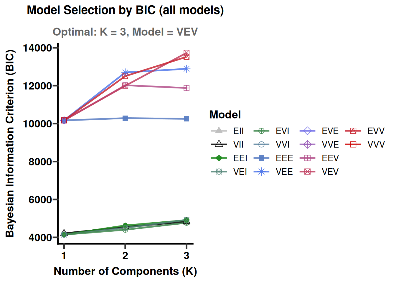
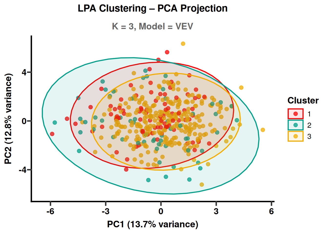
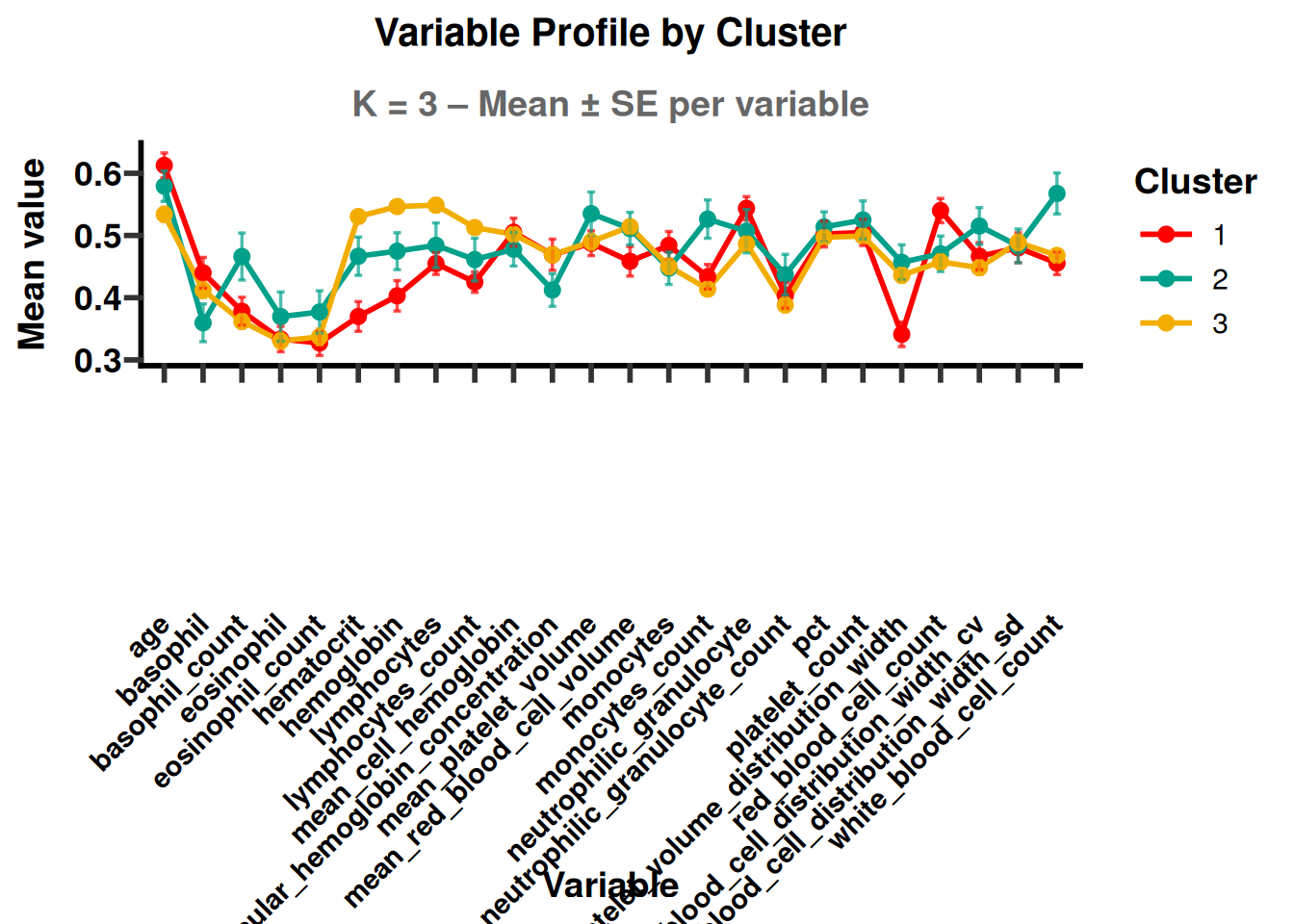
  sub_train, use_scaled_data = TRUE, max_clusters = 3, verbose = TRUE,
  color_palette = "Darjeeling1", save_plots = TRUE, save_dir = sub_dir("02_lpa"), seed = SEED
)
cat("LPA optimal K =", sub_train@Optimal.cluster, "\n")
print(table(sub_train@info.data$cluster_lpa))
## 3.3 NMF (Non-negative Matrix Factorization) — the primary method here,
## because it produces a re-usable model that can assign new/validation
## samples to the same subtypes (steps 3.3d and 4 below).
cat("\n=== NMF Clustering ===\n")
library(NMF)
nmf_dir <- sub_dir("03_nmf")
````
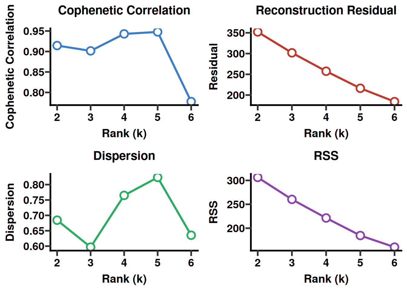
### 3.3a Estimate the best rank (= number of subtypes) across a candidate range.
This section performs the core analysis for this stage. Review the output immediately below the code and confirm that data ranges, assumptions, and results match the study design.
````{r}
#| label: module3-advanced-14
#| echo: true
#| message: false
#| warning: false
#| fig-show: hold
#| out-width: '100%'
# 3.3a Estimate the best rank (= number of subtypes) across a candidate range.
sub_train <- Sub_nmf_estimate(sub_train, rank_range = 2:6, nrun = 5,
                              method = "brunet", save_dir = nmf_dir, seed = SEED)
````
### 3.3b Pick the best rank from the estimation above.
This section performs the core analysis for this stage. Review the output immediately below the code and confirm that data ranges, assumptions, and results match the study design.
````{r}
#| label: module3-advanced-15
#| echo: true
#| message: false
#| warning: false
#| fig-show: hold
#| out-width: '100%'
# 3.3b Pick the best rank from the estimation above.
sub_train <- Sub_nmf_best_rank(sub_train, nrun = 5, method = "brunet",
                               palette_name = "Zissou1", save_dir = nmf_dir)
cat("NMF optimal rank =", sub_train@Optimal.cluster, "\n")
````
### 3.3c Assign each training sample to a subtype.
This section trains and compares candidate models. Select models using discrimination, calibration, stability, and clinical utility together.
````{r}
#| label: module3-advanced-16
#| echo: true
#| message: false
#| warning: false
#| fig-show: hold
#| out-width: '100%'
# 3.3c Assign each training sample to a subtype.
sub_train <- Sub_nmf_assign_subtypes(sub_train)
print(table(sub_train@info.data$cluster_nmf))
````
### 3.3d Refit with more NMF runs and save a re-usable model object for new data
This section trains and compares candidate models. Select models using discrimination, calibration, stability, and clinical utility together.
````{r}
#| label: module3-advanced-17
#| echo: true
#| message: false
#| warning: false
#| fig-show: hold
#| out-width: '100%'
# 3.3d Refit with more NMF runs and save a re-usable model object, so new
# samples (or the validation split) can be classified consistently later.
model_dir <- sub_dir("03_nmf/model")
sub_train <- Sub_nmf_train_model(
  sub_train, best_k = sub_train@Optimal.cluster, nrun = 10, method = "brunet",
  model_name = "subtyping_nmf_model", save_dir = model_dir
)
# =============================================================================
````
### 4 Predict Subtypes on the Validation Split
This section creates training and validation sets. Restrict feature selection and parameter estimation to the training set to prevent leakage.
````{r}
#| label: module3-advanced-18
#| echo: true
#| message: false
#| warning: false
#| fig-show: hold
#| out-width: '100%'
# 4. Predict Subtypes on the Validation Split
# =============================================================================
cat("\n=== Predict validation set using the trained NMF model ===\n")
sub_test <- Sub_predict_subtypes(sub_test, train_object = sub_train, method = "nmf", verbose = TRUE)
cat("Validation NMF subtype distribution:\n")
print(table(sub_test@info.data$cluster_nmf))
# =============================================================================
````
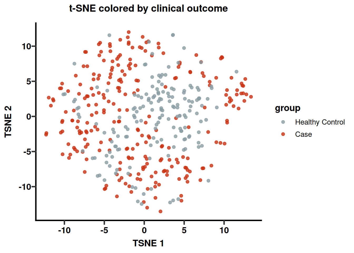
### 5 Dimensionality Reduction for Visualization (t-SNE & UMAP)
This section creates exploratory and reporting figures. Plots appear below the code and are also saved as vector PDFs for publication.
````{r}
#| label: module3-advanced-19
#| echo: true
#| message: false
#| warning: false
#| fig-show: hold
#| out-width: '100%'
# 5. Dimensionality Reduction for Visualization (t-SNE & UMAP)
# =============================================================================
cat("\n=== Dimensionality reduction (t-SNE & UMAP) ===\n")
dr_dir <- sub_dir("04_dim_reduction")

sub_train <- Sub_tsne_analyse(sub_train, use_scaled_data = TRUE)
sub_train <- Sub_umap_analyse(sub_train, n_neighbors = 15, min_dist = 0.1, metric = "euclidean")
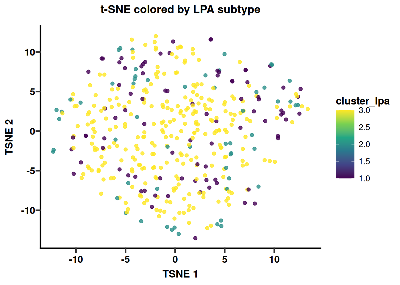
# t-SNE colored by LPA subtype.
PlotDimReduction(sub_train, reduction = "tsne", color_by = "cluster_lpa",
                 palette_name = "Darjeeling1", save_plot = TRUE,
                 save_dir = file.path(dr_dir, "tsne"), point_size = 1.8) +
  ggplot2::labs(title = "t-SNE colored by LPA subtype")
# t-SNE colored by the clinical outcome (as a factor for discrete coloring).
sub_train@info.data[[GROUP_COL]] <- factor(sub_train@info.data[[GROUP_COL]])
PlotDimReduction(sub_train, reduction = "tsne", color_by = GROUP_COL,
                 palette_name = "Royal1", save_plot = TRUE,
                 save_dir = file.path(dr_dir, "tsne"), point_size = 1.8) +
  ggplot2::labs(title = "t-SNE colored by clinical outcome")
# =============================================================================
````
### 6 Clustering Quality Evaluation
This section evaluates quality and robustness. Interpret plots, metrics, and sample distributions together.
````{r}
#| label: module3-advanced-20
#| echo: true
#| message: false
#| warning: false
#| fig-show: hold
#| out-width: '100%'
# 6. Clustering Quality Evaluation
# =============================================================================
cat("\n=== Clustering quality evaluation ===\n")
# Use a separate temporary copy per method so none of them overwrite each other.
km_eval  <- sub_train; km_eval@clustered.data$group  <- sub_train@info.data$cluster_kmeans
lpa_eval <- sub_train; lpa_eval@clustered.data$group <- sub_train@info.data$cluster_lpa
nmf_eval <- sub_train; nmf_eval@clustered.data$group <- sub_train@info.data$cluster_nmf

eval_km  <- Sub_evaluation_results(km_eval,  seed = SEED)
eval_lpa <- Sub_evaluation_results(lpa_eval, seed = SEED)
eval_nmf <- Sub_evaluation_results(nmf_eval, seed = SEED)
eval_summary <- data.frame(
  Method = c("K-means", "LPA", "NMF"),
  rbind(eval_km@evaluation_results, eval_lpa@evaluation_results, eval_nmf@evaluation_results)
)
print(eval_summary)
# =============================================================================
````
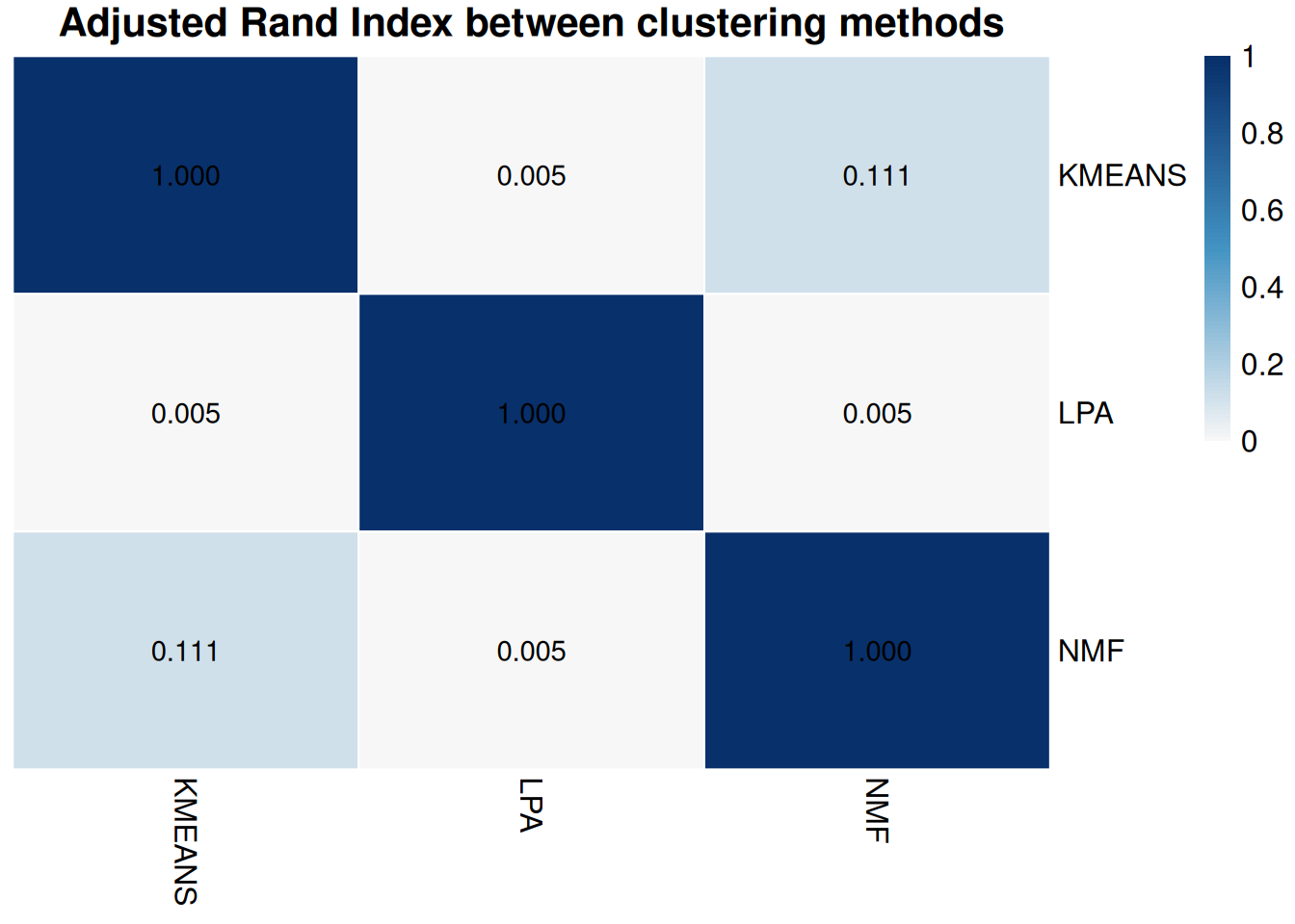
### 7 Consistency Between the Three Clustering Methods
This section evaluates quality and robustness. Interpret plots, metrics, and sample distributions together.
````{r}
#| label: module3-advanced-21
#| echo: true
#| message: false
#| warning: false
#| fig-show: hold
#| out-width: '100%'
# 7. Consistency Between the Three Clustering Methods
# =============================================================================
cat("\n=== Consistency between methods ===\n")
sub_compare <- sub_train
# Prefix numeric cluster labels with "S" so they are treated as categories,
# not as an ordered numeric scale, in the comparison plot.
sub_compare@info.data$cluster_lpa    <- paste0("S", sub_compare@info.data$cluster_lpa)
sub_compare@info.data$cluster_kmeans <- paste0("S", sub_compare@info.data$cluster_kmeans)

ari_mat <- compare_clusterings(
  sub_compare, methods = c("cluster_kmeans", "cluster_lpa", "cluster_nmf"), output = "matrix"
)
cat("Adjusted Rand Index matrix:\n"); print(round(ari_mat, 3))
plot_clustering_comparison(
  sub_compare, methods = c("cluster_kmeans", "cluster_lpa", "cluster_nmf"),
  save_dir = sub_dir("05_method_comparison"), width = 5, height = 4.5, base_size = 12
)
# =============================================================================
````
### 8 Subtype-Specific Marker Features & Enhanced Visualization
This section creates exploratory and reporting figures. Plots appear below the code and are also saved as vector PDFs for publication.
````{r}
#| label: module3-advanced-22
#| echo: true
#| message: false
#| warning: false
#| fig-show: hold
#| out-width: '100%'
# 8. Subtype-Specific Marker Features & Enhanced Visualization
# =============================================================================
cat("\n=== Subtype-specific differential features ===\n")
deg_dir <- sub_dir("06_differential")

## 8.1 Multi-class differential analysis (one-vs-rest Wilcoxon), using the
## LPA subtypes as the grouping variable. Any of the three cluster labels
## could be used here instead.
deg_df <- sub_train@clean.data
deg_df$subtype <- factor(sub_train@info.data$cluster_lpa)

multi_deg <- batch_Wilcoxon_MultiClass(
  mat = deg_df, group_col = "subtype", only.pos = FALSE,
  save_data = TRUE, save_dir = deg_dir
)
## 8.2 Marker heatmaps of the top differential features per subtype.
# Basic version, auto z-limit:
tryCatch(
  PlotClusterHeatmap(
    sub_train, p_cutoff = 2, deg_df = multi_deg, top_n = 5,
    save_path = file.path(deg_dir, "cluster_heatmap_basic.pdf")
  ),
  error = function(e) message("Sample-level heatmap skipped (raster backend): ", e$message)
)
# With a clinical annotation bar (outcome) alongside the heatmap:
tryCatch(
  PlotClusterHeatmap(
    sub_train, p_cutoff = 2, deg_df = multi_deg, group_by = "cluster_lpa",
    annotation_cols = tolower(GROUP_COL), top_n = 5, log_transform = TRUE,
    save_path = file.path(deg_dir, "cluster_heatmap_with_outcome.pdf"),
    # Key the palette by the SAME name as annotation_cols. A key that does not
    # match an annotation column is ignored silently, so the bar comes out in
    # the default colours instead of failing loudly.
    annotation_palette = setNames(
      list(c("Case" = "#D32F2F", "Healthy Control" = "#1976D2")),
      tolower(GROUP_COL))
  ),
  error = function(e) message("Annotated sample-level heatmap skipped (raster backend): ", e$message)
)
# Group-mean z-score heatmap (one column per subtype, not per sample) —
# useful for a compact summary figure.
PlotGroupMeanHeatmap(
  sub_train, deg_df = multi_deg, top_n = 5, custom_levels = c("1", "2", "3"),
  z_score_type = "row", heatmap_palette = c("#2166AC", "white", "#B2182B"),
  save_path = file.path(deg_dir, "group_mean_zscore.pdf")
)

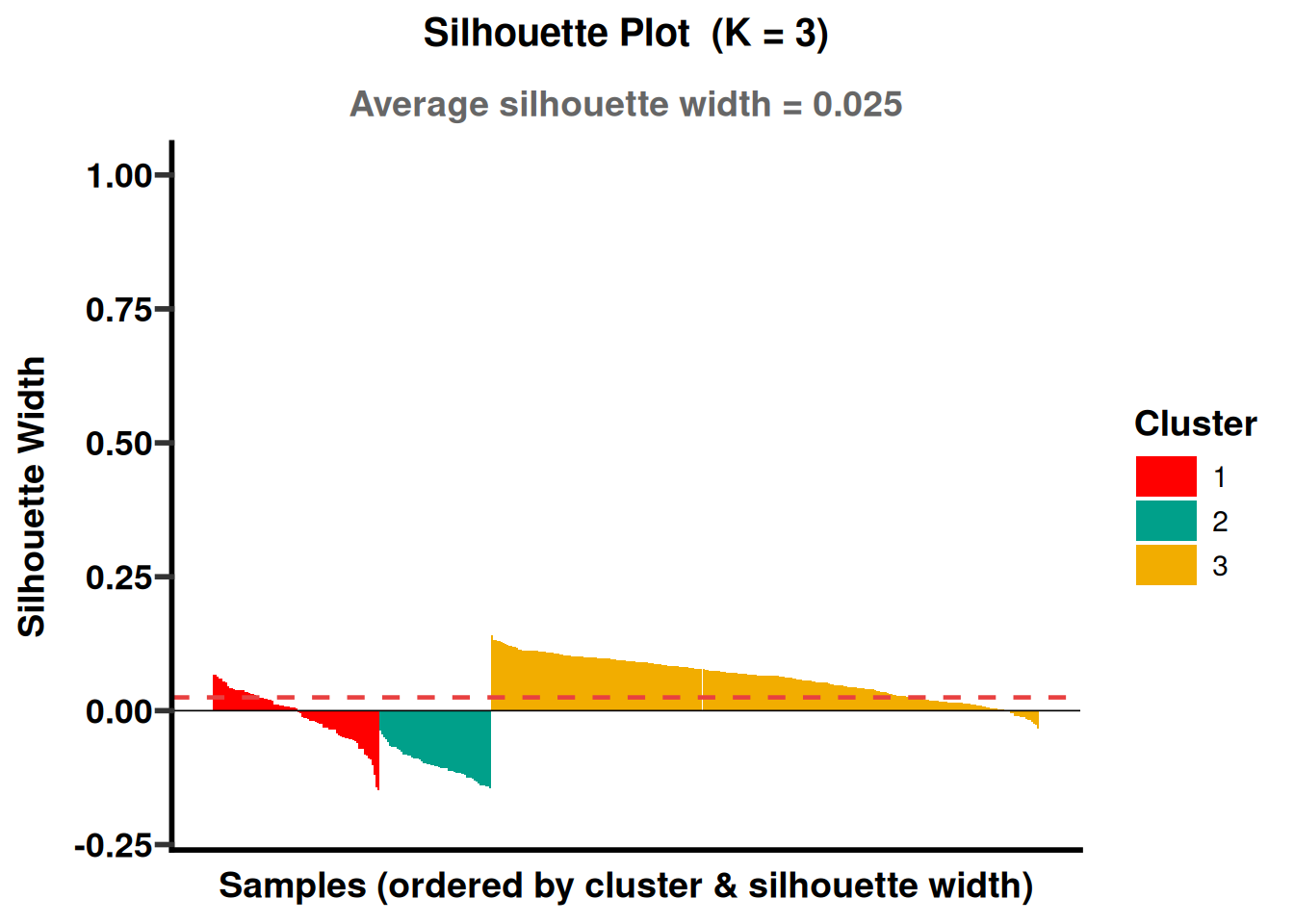
## 8.3 Silhouette plot — how well-separated are the LPA subtypes?
PlotSilhouette(sub_train, group_by = "cluster_lpa", dist_method = "euclidean",
               palette_name = "Darjeeling1", save_plot = TRUE, save_dir = sub_dir("07_silhouette"))

## 8.4 Alluvial diagram comparing outcome, K-means, LPA, and NMF assignments
## for the same samples — a compact way to show whether methods agree.
PlotMultiAlluvial(
  sub_train, cols_list = c(tolower(GROUP_COL), "cluster_kmeans", "cluster_lpa", "cluster_nmf"),
  save_plot = TRUE, save_dir = sub_dir("08_alluvial")
)

# =============================================================================
````
### 9 Deployment: Predict Subtypes for New Samples
This section applies the trained object to new samples. Validate input format, performance, and target population in an independent cohort before deployment.
````{r}
#| label: module3-advanced-23
#| echo: true
#| message: false
#| warning: false
#| fig-show: hold
#| out-width: '100%'
# 9. Deployment: Predict Subtypes for New Samples
# =============================================================================
demo_raw_data <- head(sub_train@clean.data, 20)
sub_manager   <- New_Sub_Manager(sub_train)

# Console-only prediction (no UI) for a quick sanity check.
quick_pred <- sub_manager$sub_predict(head(demo_raw_data), method = "nmf")
print(quick_pred@info.data$cluster_nmf)
# Optional metadata shown in the deployment app.
my_intro <- list(
  abstract = "Cohort-scale subtyping tool.",
  citation = "Add your citation here."
)
my_var_dict <- data.frame(
  Feature     = c("gender", "age", "wbc", "platelets", "crp", "ldh"),
  Description = c("Patient biological sex (1 = Male, 2 = Female)",
                  "Patient age at diagnosis",
                  "White blood cell count",
                  "Total platelet count",
                  "C-reactive protein (inflammation marker)",
                  "Lactate dehydrogenase (tumor-burden marker)"),
  Units       = c("Category", "Years", "10^9/L", "10^9/L", "mg/L", "U/L"),
  stringsAsFactors = FALSE
)

# The interactive Shiny app is only launched in an interactive session.
if (interactive()) {
  launch_sub_deploy_app(sub_manager, var_dict = my_var_dict,
                        title = "Stratification Portal", project_info = my_intro)
}

# =============================================================================
````
### 10 Save Final Objects
This section saves model objects, tables, and figures for reproducibility, review, and reuse.
````{r}
#| label: module3-advanced-24
#| echo: true
#| message: false
#| warning: false
#| fig-show: hold
#| out-width: '100%'
# 10. Save Final Objects
# =============================================================================
saveRDS(sub_train, file = file.path(OUTPUT_DIR, "final_subtyping_object.rds"))

cat("\n========================================\n")
cat("Module 3 (advanced) pipeline finished successfully!\n")
cat("Optimal cluster numbers — K-means:", eval_km@evaluation_results$n_clusters,
    "| LPA:", eval_lpa@evaluation_results$n_clusters,
    "| NMF:", eval_nmf@evaluation_results$n_clusters, "\n")
cat("Best method by Silhouette score:", eval_summary$Method[which.max(eval_summary$Silhouette)], "\n")
cat("All results saved under:", OUTPUT_DIR, "\n")
cat("========================================\n")
````