# Module 1: Data Cleaning and Exploration — Quick Start
This chapter introduces the official `Stat` workflow: import an Excel cohort, create an object with `CreateStatObject()`, inspect variable types and data quality, clean and normalize the predictors, visualize group structure, test group differences, and create a publication-oriented Table 1. The saved `stat_obj.rds` retains the processed data and transformation state for Modules 2 and 3.
## When to Use This Chapter
Use this chapter for a reproducible first pass through clinical or omics data. Confirm the inferred variable types and missing-data assumptions before accepting automated cleaning. Use the advanced chapter when the study requires comprehensive diagnostics, explicit outlier handling, differential-feature analysis, or manuscript figures.
## Step-by-step Workflow
<!-- split-into-step-chunks -->
The workflow is divided into short stages. Each note explains the purpose, key checks, and interpretation limits. Generated plots and tables appear directly below their code chunk.
### Environment and Global Setup
This section performs the core analysis for this stage. Review the output immediately below the code and confirm that data ranges, assumptions, and results match the study design.
````{r}
#| label: module1-quickstart-01
#| cache: false
#| echo: true
#| message: false
#| warning: false
#| fig-show: hold
#| out-width: '100%'
# =============================================================================
# icare Package Vignette — Module 1: Data Cleaning & Exploratory Analysis
# QUICK-START EDITION
# =============================================================================
# Audience : First-time users, or anyone who wants a working, minimal
#            analysis in a few minutes without touching every option.
# This script covers the core workflow only:
#   load data -> create a StatObject -> clean it -> look at one or two
#   summary plots -> run a group comparison -> get a baseline table.
#
# Looking for every option, publication-ready figures, or more diagnostics?
# See "01_module1_data_cleaning_ADVANCED.R" instead.
options(warn = -1)
# =============================================================================
rm(list = ls())
library(icare)
# ---------------------------------------------------------------------------
````
### 1 Load the data
This section imports and organizes the data. Check dimensions and variable coding before continuing.
````{r}
#| label: module1-quickstart-02
#| echo: true
#| message: false
#| warning: false
#| fig-show: hold
#| out-width: '100%'
# 1. Load the data
# ---------------------------------------------------------------------------
library(readxl)
raw_dis=as.data.frame(read_excel("data/PMID37633276_DIA_plasmaproomic.xlsx",sheet = 3))
raw_dis=raw_dis[!grepl(x = raw_dis$`Case ID`,pattern = "^KC"),]
dput(colnames(raw_dis))
mat=raw_dis[,c( "White blood cell count",
               "Lymphocytes%", "Monocytes%", "Neutrophilic granulocyte%", "Eosinophil%",
               "Basophil%", "Lymphocytes count", "Monocytes count", "Neutrophilic granulocyte count",
               "Eosinophil count", "Basophil count", "Red blood cell count",
               "Hemoglobin", "Hematocrit", "Mean red blood cell volume", "Mean cell hemoglobin",
               "Mean corpuscular hemoglobin concentration", "Red blood cell distribution width CV",
               "Red blood cell distribution width SD", "Platelet count", "Mean platelet volume",
               "PCT", "Platelet volume distribution width")]
index=grepl(x = raw_dis$`Case ID`,pattern = "^HC")
inf=raw_dis[,c("Case ID", "Sample type", "Plasma proteome ID", "Tissue proteome ID",
      "Gender", "Age at diagnosis", "Tobacco smoking history", "Drinking history",
      "Vital status", "Days to last followup", "Days until death",
      "Combined days to last followup or death", "Progressive-free survival_Status",
      "Progressive-free survival_Months", "Tumor location", "Tumor size (cm)",
      "T-category", "Lymph node involvement", "Distant metastasis",
      "TNM Stage", "Grade", "Morphology")]
# The group label goes in `inf` ONLY. icare stores the label in info.data and
# keeps it out of the feature matrix entirely: a label sitting among the
# features is indistinguishable from a feature to any code that selects columns
# by type, and a numeric 0/1 label would silently be fed into PCA and the
# correlation heatmap. Because the label never enters `mat`, its R type is free
# -- labels can be readable strings, which is what you want in the Table 1
# column headers.
inf$group = factor(ifelse(index, "Healthy Control", "Case"),
                   levels = c("Healthy Control", "Case"))

# `mat` stays purely numeric, so as.matrix()/storage.mode() is a safe no-op and
# any non-numeric column here would be a genuine mistake rather than a silent NA.
mat=as.matrix(mat)
storage.mode(mat) <- "numeric"

rownames(mat)=inf$`Case ID`
rownames(inf)=inf$`Case ID`
# ---------------------------------------------------------------------------
````
### 2 Create the Stat object
This section creates the icare analysis object that stores data, metadata, and workflow state for all later steps.
````{r}
#| label: module1-quickstart-03
#| echo: true
#| message: false
#| warning: false
#| fig-show: hold
#| out-width: '100%'
# 2. Create the Stat object
# ---------------------------------------------------------------------------
# This is the container icare uses to track your data through cleaning.
# group_col tells icare which column is the outcome you want to compare groups on.
stat_obj <- CreateStatObject(
  raw.data  = mat,info.data = inf,
  group_col = "group",
  na.action = "allow"
)
# ---------------------------------------------------------------------------
````
### 3 Clean the data (one line per step, sensible defaults)
This section preprocesses the data. Review missingness, outlier handling, and normalization before accepting the defaults.
````{r}
#| label: module1-quickstart-04
#| echo: true
#| message: false
#| warning: false
#| fig-show: hold
#| out-width: '100%'
# 3. Clean the data (one line per step, sensible defaults)
# ---------------------------------------------------------------------------
stat_obj <- stat_diagnose_variable_type(stat_obj)          # detect numeric vs. categorical
stat_obj <- stat_convert_variables(stat_obj) # apply those types
stat_obj <- stat_miss_processed(stat_obj, impute_method = "median_mode") # fill missing values
stat_obj <- stat_detect_and_mark_outliers(stat_obj, method = "iqr") # flag outliers
stat_obj <- stat_handle_outliers(stat_obj, method = "impute", impute_value = "median") # fix them
stat_obj <- stat_onehot_encode(stat_obj) # encode categorical variables
stat_obj <- stat_normalize_process(stat_obj, method = "auto") # normalize numeric variables
cat("Clean data ready:", nrow(stat_obj@clean.data), "rows x",
    ncol(stat_obj@clean.data), "columns\n")
# ---------------------------------------------------------------------------
````
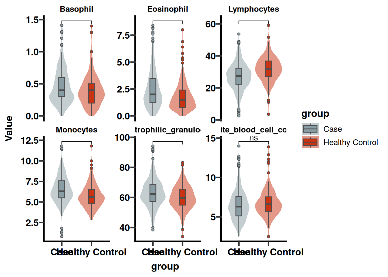
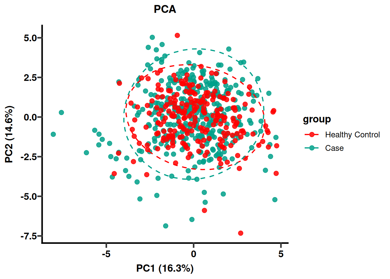
### 4 Two quick summary plots
This section creates exploratory and reporting figures. Plots appear below the code and are also saved as vector PDFs for publication.
````{r}
#| label: module1-quickstart-05
#| echo: true
#| message: false
#| warning: false
#| fig-show: hold
#| out-width: '100%'
# 4. Two quick summary plots
# ---------------------------------------------------------------------------
# A) How do the groups differ across a few key numeric variables?
numeric_vars <- names(stat_obj@clean.data)[sapply(stat_obj@clean.data, is.numeric)]
PlotGroupedDistribution(
  object    = stat_obj,
  features  = head(numeric_vars, 6),
  group_col = "group",
  test      = "wilcox.test",
  save_plot = TRUE
)
# B) Do the two groups separate overall (PCA)?
PlotPCA(
  object   = stat_obj,
  color_by = "group",
  ellipse  = TRUE,
  save_plot = TRUE
)
# ---------------------------------------------------------------------------
````
### 5 Which features differ most between groups?
This section selects candidate features. Consider effect size, stability, and biological plausibility rather than a single significance measure.
````{r}
#| label: module1-quickstart-06
#| echo: true
#| message: false
#| warning: false
#| fig-show: hold
#| out-width: '100%'
# 5. Which features differ most between groups?
# ---------------------------------------------------------------------------
stat_obj <- stat_var_feature(stat_obj, p_threshold = 0.05)
deg_result <- ExtractLastTestSig(stat_obj)
# ---------------------------------------------------------------------------
````
### 6 Baseline characteristics table ("Table 1")
This section performs the core analysis for this stage. Review the output immediately below the code and confirm that data ranges, assumptions, and results match the study design.
````{r}
#| label: module1-quickstart-07
#| echo: true
#| message: false
#| warning: false
#| fig-show: hold
#| out-width: '100%'
# 6. Baseline characteristics table ("Table 1")
# ---------------------------------------------------------------------------
stat_obj <- stat_gaze_analysis(stat_obj, save_word = TRUE)
# ---------------------------------------------------------------------------
````
### 7 Save your work
This section saves model objects, tables, and figures for reproducibility, review, and reuse.
````{r}
#| label: module1-quickstart-08
#| echo: true
#| message: false
#| warning: false
#| fig-show: hold
#| out-width: '100%'
# 7. Save your work
# ---------------------------------------------------------------------------
# Module 2 (modeling) and Module 3 (subtyping) both can start by loading this file.
saveRDS(stat_obj, file = "stat_obj.rds")

cat("\nDone! stat_obj.rds saved — you're ready for Module 2 (modeling)",
    "or Module 3 (subtyping).\n")
````