1The first complete workflow: ORA, GSEA, and plots
This chapter starts from the committed datasets/de_table.tsv file derived from the Bioconductor airway example with DESeq2. The table contains Ensembl IDs, differential-expression statistics, and adjusted p-values for dexamethasone-treated versus untreated airway smooth-muscle samples. The table is local at render time; the regeneration script and package provenance are documented in datasets/readme.md.
The example answers two related questions about the same contrast:
ORA: among genes selected by an explicit adjusted-p-value and fold-change rule, which biological-process terms are over-represented?
GSEA: across the complete DESeq2 Wald-statistic ranking, which terms are shifted toward the top or bottom?
The thresholds are teaching choices. In a real analysis, replace them with rules defined before inspecting enrichment results.
    baseMean         log2FoldChange           stat                padj
 Min.   :     0.00   Min.   :-5.325905   Min.   :-19.41608   Min.   :0.0000
 1st Qu.:     0.00   1st Qu.:-0.463691   1st Qu.: -0.56367   1st Qu.:0.6952
 Median :     0.11   Median :-0.014700   Median : -0.03119   Median :0.9963
 Mean   :   336.15   Mean   :-0.008159   Mean   :  0.05032   Mean   :0.7853
 3rd Qu.:    10.28   3rd Qu.: 0.381747   3rd Qu.:  0.48069   3rd Qu.:0.9963
 Max.   :325662.66   Max.   : 9.505972   Max.   : 24.85609   Max.   :0.9999
                     NAs    :30208       NAs    :30208       NAs    :30208
The table uses Ensembl gene IDs and the stat column supplies a signed ranking. Keep both facts visible in an analysis script. An identifier can be syntactically valid and still be incompatible with the selected annotation database.
1.2 2. Define the universe, selected genes, and ranking
The ORA universe starts with genes having a finite DESeq2 statistic and is then restricted to Ensembl IDs present in org.Hs.eg.db. The selected list applies a fixed padj and absolute log2 fold-change rule. GSEA uses the complete finite, mapped statistic ranking, including genes that do not pass the ORA threshold.
cat("Selected genes for ORA:", length(selected), "\n")
Selected genes for ORA: 885
cat("Selected genes in universe:", all(selected %in% universe), "\n")
Selected genes in universe: TRUE
universe, selected, and ranking use the same Ensembl namespace after filtering against the keys available in org.Hs.eg.db. The unmapped count is reported rather than silently treated as biological absence. In a real experiment, construct the candidate universe from genes that were measurable and eligible for selection, then record the annotation coverage.
1.3 3. Run over-representation analysis
enrichGO() tests Gene Ontology terms using the selected vector. ont = "BP" restricts this example to biological process terms; use "MF", "CC", or "ALL" when that choice matches the question. The permissive pvalueCutoff = 1 and qvalueCutoff = 1 settings keep the complete result object for teaching and plotting; apply a pre-specified reporting threshold when interpreting a real study.
The output is an enrichResult. Its @result slot can be converted to a data frame, but retain ora itself: the object carries the gene-to-term information needed by downstream plots.
enrichGO() accepts the Ensembl input but uses an Entrez-backed annotation internally when that is memory-efficient; the returned object preserves the original input key type (ENSEMBL). Readable symbols can be added for inspection without changing the test. Let setReadable() use the key type recorded on the result object:
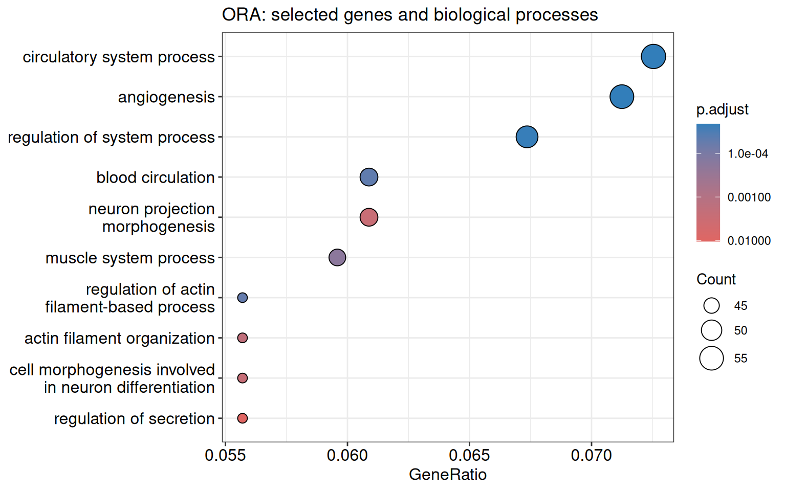
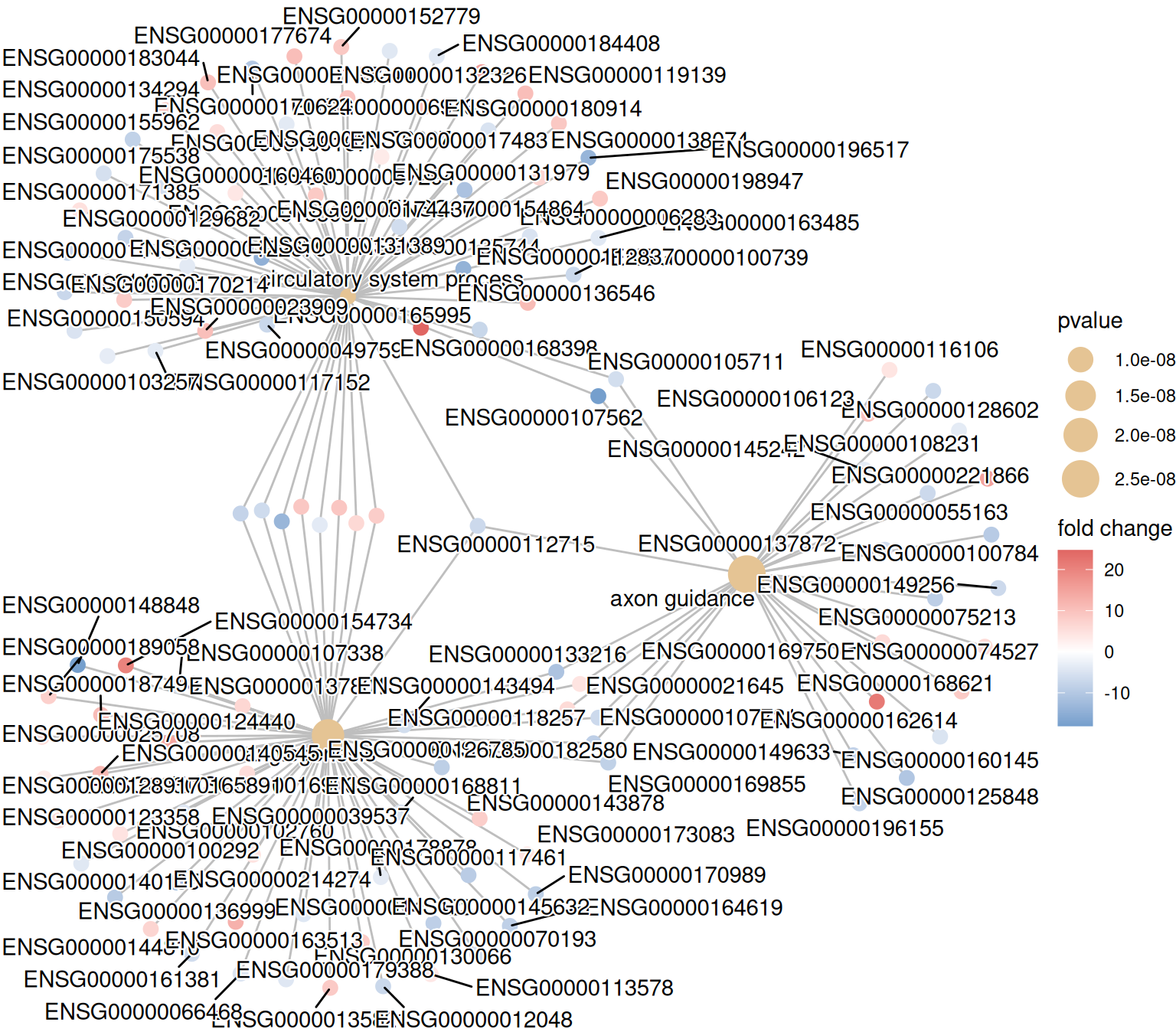
A dot plot is a compact first view. Dot size is the number of selected genes in a term, and colour represents the adjusted significance used by the plotting method. A network plot is useful for seeing shared genes among a small number of terms.
p_ora_dot <-dotplot(ora, showCategory =10) +ggtitle("ORA: selected genes and biological processes")p_ora_dot
cnetplot() is intentionally limited to three terms here. Showing every term usually produces a dense graph that is harder to read than the dot plot.
1.5 5. Run GSEA on the complete ranking
GSEA does not use selected as its input. It uses the complete named ranking, so genes below the ORA threshold still contribute. The minGSSize and maxGSSize settings keep this first local example reasonably quick while excluding extremely small or very broad terms.
NoteSize filter is on the overlap, not the raw gene set
minGSSize and maxGSSize constrain the size of each gene set after intersecting with the genes present in your ranking (names(geneList)). A database gene set with 3 000 annotated members is therefore not dropped just because 3 000 > maxGSSize = 500; it is retained if only 400 of its members appear in the ranked list. Full rationale and tuning tables are in Tuning minGSSize and maxGSSize.
Setting cutoffs to 1 retains the tested terms so that the plotting example remains informative even when few terms meet a conventional significance threshold.
The result is a gseaResult. Its NES and enrichmentScore describe direction and magnitude relative to the ranked list; the adjusted p-value controls for testing many terms. Inspect both effect direction and statistical evidence rather than sorting only by a single column.
1.6 6. Visualize the GSEA result
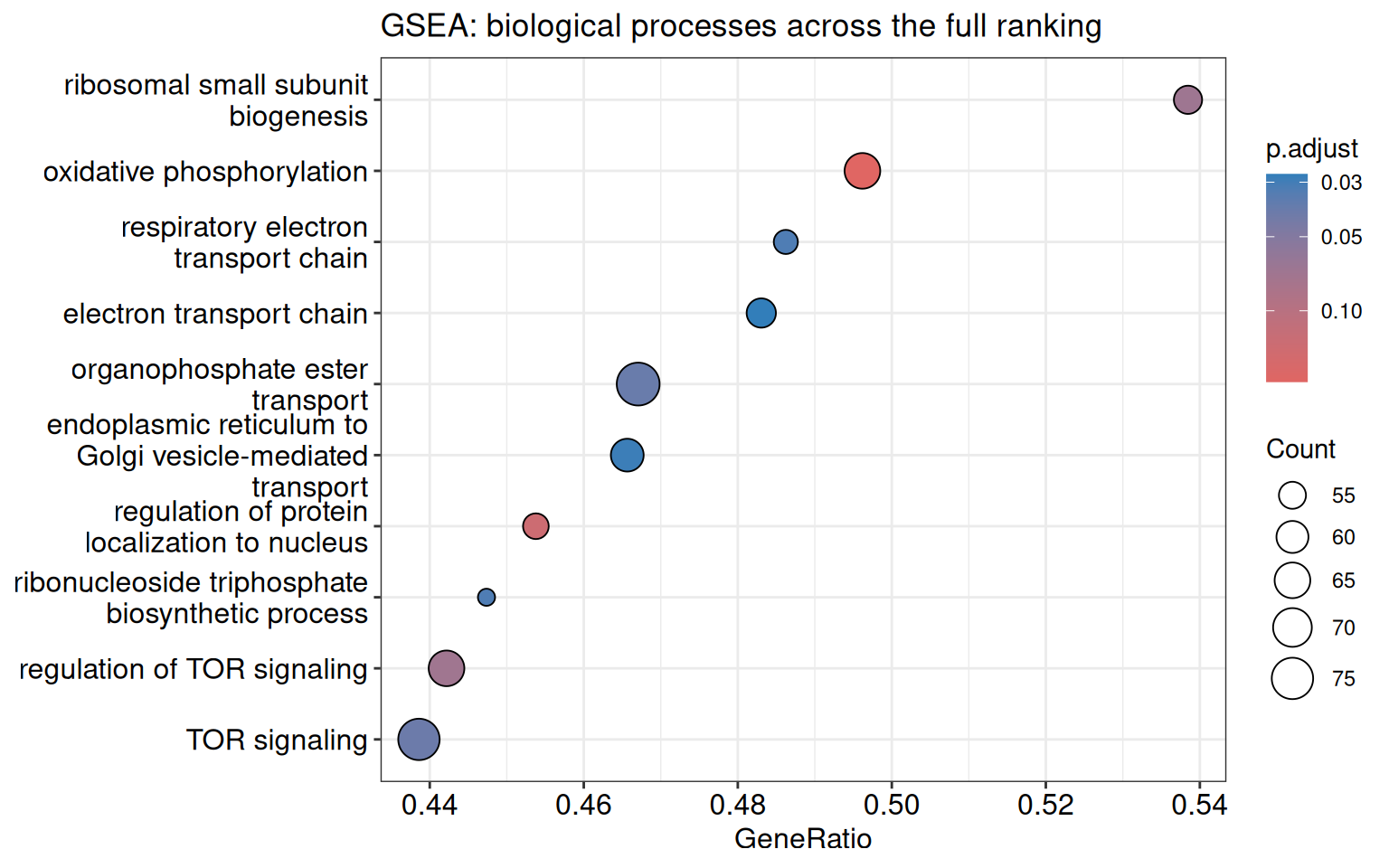
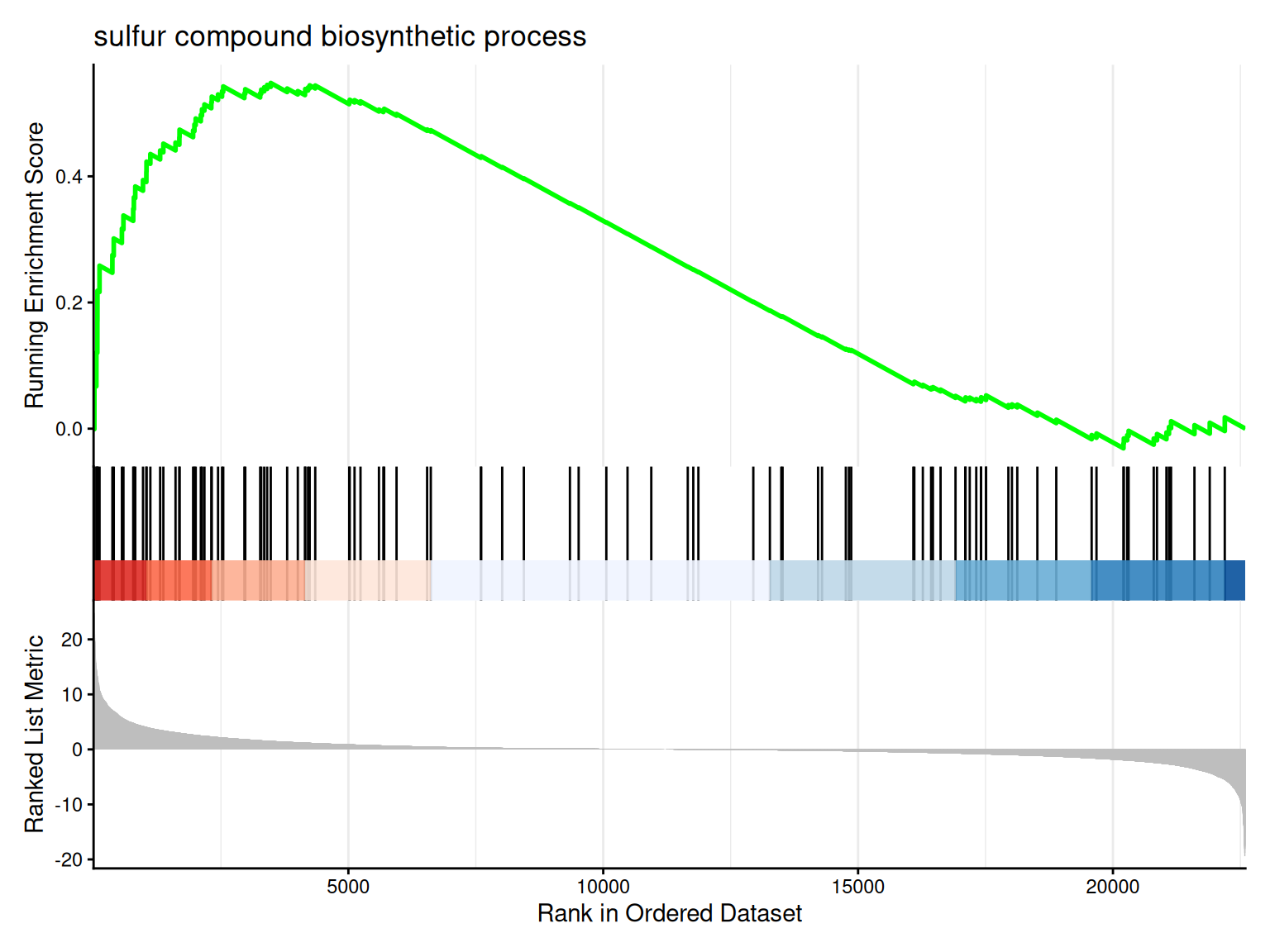
The dot plot gives a profile-level overview. gseaplot2() shows the running enrichment score, the locations of genes in the selected set, and the ranked statistic for one term.
p_gsea_dot <-dotplot(gsea, showCategory =10) +ggtitle("GSEA: biological processes across the full ranking")p_gsea_dot
if (nrow(as.data.frame(gsea)) >0) {gseaplot2(gsea, geneSetID =1, title = gsea$Description[1])}
The x-axis of a GSEA curve is the position in the ranked list, not a gene identifier. A term enriched at the top has a positive direction for this signed ranking; a term enriched at the bottom has a negative direction.
1.7 7. Compare the two questions and save results
ORA and GSEA can both be useful, but they are not duplicate tests. ORA asks whether a thresholded set has more members of a term than expected under the universe. GSEA asks whether term members accumulate toward one end of the complete ranking. Report which input and background were used for each result.
# These files are optional outputs; the result objects remain the analysis record.write.csv(de_table, "de-table-used.csv", row.names =FALSE)write.csv(as.data.frame(ora_readable), "ora-go-bp-results.csv", row.names =FALSE)write.csv(as.data.frame(gsea), "gsea-go-bp-results.csv", row.names =FALSE)saveRDS(list(input = de_table,universe = universe,selected = selected,ranking = ranking,ora = ora,gsea = gsea ),"enrichment-objects.rds")
For a short report, start with the two dot plots and one GSEA curve. For a detailed report, include the ID type, universe construction, threshold, ontology, package versions, and the complete result tables.
Offline boundary. This chapter uses data shipped with R/Bioconductor packages. org.Hs.eg.db is a local annotation package, and the example does not query KEGG, Enrichr, g:Profiler, or another remote service. A real study should record the annotation package version because local annotations change over time.