8 Annotating Tree with Silhouette Images and Sub-plots

8.1 Annotating Tree with Images

We usually use text to label taxa, i.e. displaying taxa names. If the text is the image file name (either local or remote), ggtree can read the image and display the actual image as the label of the taxa (Figure 8.1). The geom_tiplab() and geom_nodelab() are capable to render silhouette images with supports from in-house developed package, ggimage.

Online tools such as iTOL (Letunic & Bork, 2007) and EvolView (He et al., 2016) support displaying subplots on a phylogenetic tree. However, only bar and pie charts are supported by these tools. Users may want to visualize node-associated data with other visualization methods, such as violin plot (Grubaugh et al., 2017), venn diagram (Lott et al., 2015), sequence logo, etc., and display them on the tree. In ggtree, all kinds of subplots are supported, as we can export all subplots to image files and use them to label corresponding nodes on the tree.

library(ggimage)
library(ggtree)

nwk <- paste0("((((bufonidae, dendrobatidae), ceratophryidae),",
          "(centrolenidae, leptodactylidae)), hylidae);")

imgdir <- system.file("extdata/frogs", package = "TDbook")

x = read.tree(text = nwk)
ggtree(x) + xlim(NA, 7) + ylim(NA, 6.2) +
    geom_tiplab(aes(image=paste0(imgdir, '/', label, '.jpg')), 
                geom="image", offset=2, align=2, size=.2)  + 
    geom_tiplab(geom='label', offset=1, hjust=.5) + 
    geom_image(x=.8, y=5.5, image=paste0(imgdir, "/frog.jpg"), size=.2)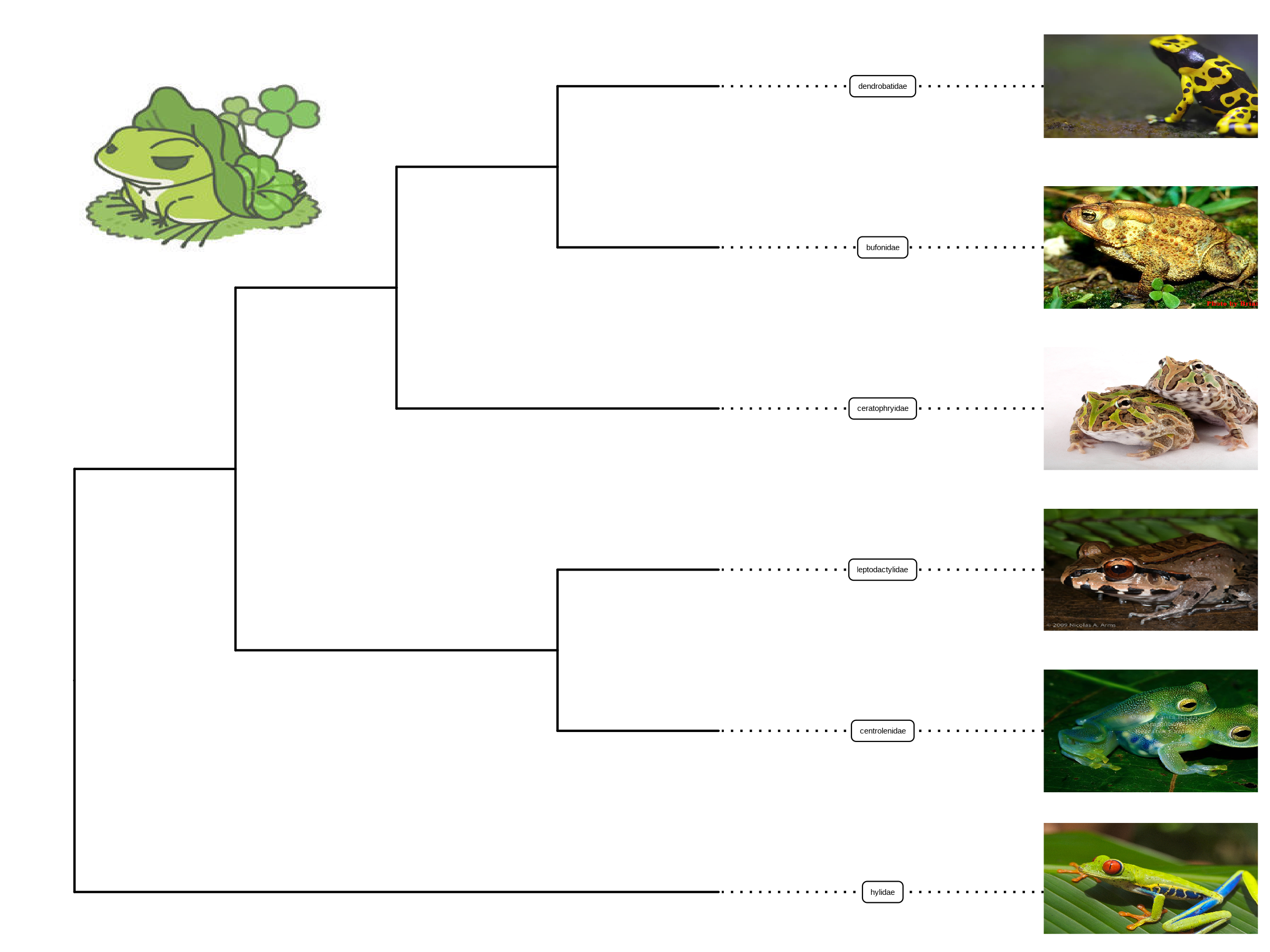

FIGURE 8.1: Labelling taxa with images. Users need to specify geom = "image" and map the image file names onto the image aesthetics.

8.2 Annotating Tree with Phylopic

Phylopic contains more than 3200 silhouettes and covers almost all life forms. The ggtree package supports using phylopic¹³ to annotate the tree by setting geom="phylopic" and mapping phylopic UID to the image aesthetics. The ggimage package supports querying phylopic UID from the scientific name, which is very handy for annotating tree with phylopic. In the following example, tip labels were used to query phylopic UID, and phylopic images were used to label the tree as another layer of tip labels. Most importantly, we can color or resize the images using numerical/categorical variables, and here the values of body mass were used to encode the color of the images (Figure 8.2).

library(ggtree)
newick <- paste0("((Pongo_abelii,(Gorilla_gorilla_gorilla,(Pan_paniscus,",
          "Pan_troglodytes)Pan,Homo_sapiens)Homininae)Hominidae,",
          "Nomascus_leucogenys)Hominoidea;")

tree <- read.tree(text=newick)

d <- ggimage::phylopic_uid(tree$tip.label)
d$body_mass <- c(52, 114, 47, 45, 58, 6)

p <- ggtree(tree) %<+% d + 
  geom_tiplab(aes(image=uid, colour=body_mass), geom="phylopic", offset=2.5) +
  geom_tiplab(aes(label=label), offset = .2) + xlim(NA, 7) +
  scale_color_viridis_c()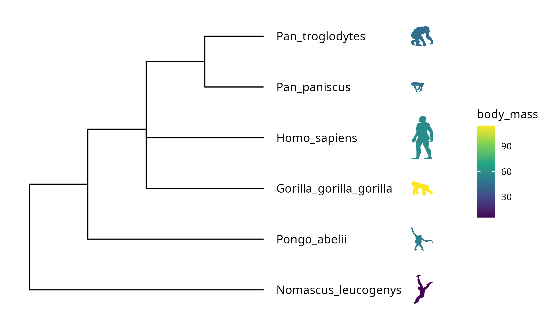

FIGURE 8.2: Labelling taxa with phylopic images. The ggtree will automatically download phylopic figures by querying provided UID. The figures can be colored using numerical or categorical values.

8.3 Annotating Tree with Sub-plots

The ggtree package provides a layer, geom_inset(), for adding subplots to a phylogenetic tree. The input is a named list of ggplot graphic objects (can be any kind of chart). These objects should be named by node numbers. Users can also use ggplotify to convert plots generated by other functions (even implemented by base graphics) to ggplot objects, which can then be used in the geom_inset() layer. To facilitate adding bar and pie charts (e.g., summarized stats of results from ancestral reconstruction) to the phylogenetic tree, ggtree provides the nodepie() and nodebar() functions to create a list of pie or bar charts.

8.3.1 Annotate with bar charts

This example uses ape::ace() function to estimate ancestral character states. The likelihoods of the stats were visualized as stacked bar charts which were overlayed onto internal nodes of the tree using the geom_inset() layer (Figure 8.3A).

library(phytools)
data(anoletree)
x <- getStates(anoletree,"tips")
tree <- anoletree

cols <- setNames(palette()[1:length(unique(x))],sort(unique(x)))
fitER <- ape::ace(x,tree,model="ER",type="discrete")
ancstats <- as.data.frame(fitER$lik.anc)
ancstats$node <- 1:tree$Nnode+Ntip(tree)

## cols parameter indicate which columns store stats
bars <- nodebar(ancstats, cols=1:6)
bars <- lapply(bars, function(g) g+scale_fill_manual(values = cols))

tree2 <- full_join(tree, data.frame(label = names(x), stat = x ), by = 'label')
p <- ggtree(tree2) + geom_tiplab() +
    geom_tippoint(aes(color = stat)) + 
    scale_color_manual(values = cols) +
    theme(legend.position = "right") + 
    xlim(NA, 8)
p1 <- p + geom_inset(bars, width = .08, height = .05, x = "branch") 

The x position can be one of ‘node’ or ‘branch’ and can be adjusted by the parameters, hjust and vjust, for horizontal and vertical adjustment, respectively. The width and height parameters restrict the size of the inset plots.

8.3.2 Annotate with pie charts

Similarly, users can use the nodepie() function to generate a list of pie charts and place these charts to annotate corresponding nodes (Figure 8.3B). Both nodebar() and nodepie() accept a parameter of alpha to allow transparency.

pies <- nodepie(ancstats, cols = 1:6)
pies <- lapply(pies, function(g) g+scale_fill_manual(values = cols))
p2 <- p + geom_inset(pies, width = .1, height = .1) 

plot_list(p1, p2, guides='collect', tag_levels='A')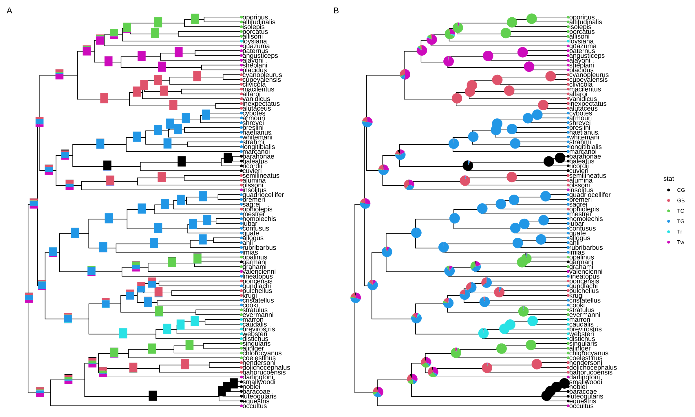

FIGURE 8.3: Annotate internal nodes with bar or pie charts. Using bar charts (A) or pie charts (B) to display summary statistics of internal nodes.

8.3.3 Annotate with mixed types of charts

The geom_inset() layer accepts a list of ‘ggplot’ graphic objects and these input objects are not restricted to pie or bar charts. They can be any kind of charts or hybrid of these charts. The geom_inset() is not only useful to display ancestral stats, but also applicable to visualize different types of data that are associated with selected nodes in the tree. Here, we use a mixture of pie and bar charts to annotate the tree as an example (Figure 8.4).

pies_and_bars <- pies
i <- sample(length(pies), 20)
pies_and_bars[i] <- bars[i]
p + geom_inset(pies_and_bars, width=.08, height=.05)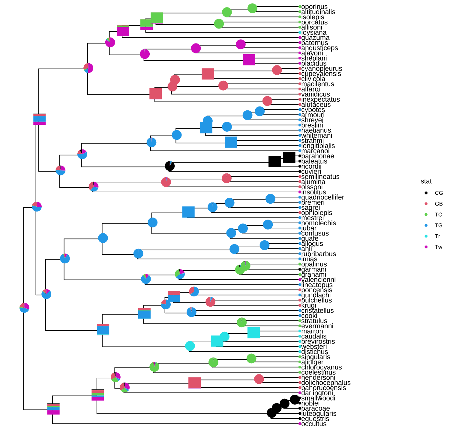

FIGURE 8.4: Annotate internal nodes with different types of subplots.

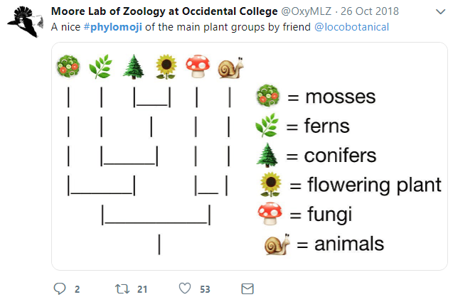
8.4 Have Fun with Phylomoji

Phylomoji is a phylogenetic tree of emoji. It is fun¹⁴ and very useful for education of the evolution concept. The ggtree supports producing phylomoji since 2015¹⁵. Here, we will use ggtree to recreate the following phylomoji figure¹⁶ (Figure 8.5):

library(ggplot2)
library(ggtree)

tt = '((snail,mushroom),(((sunflower,evergreen_tree),leaves),green_salad));'
tree = read.tree(text = tt)
d <- data.frame(label = c('snail','mushroom', 'sunflower',
                          'evergreen_tree','leaves', 'green_salad'),
                group = c('animal', 'fungi', 'flowering plant',
                          'conifers', 'ferns', 'mosses'))

p <- ggtree(tree, linetype = "dashed", size=1, color='firebrick') %<+% d + 
  xlim(0, 4.5) + ylim(0.5, 6.5) +
  geom_tiplab(parse="emoji", size=15, vjust=.25) +
  geom_tiplab(aes(label = group), geom="label", x=3.5, hjust=1)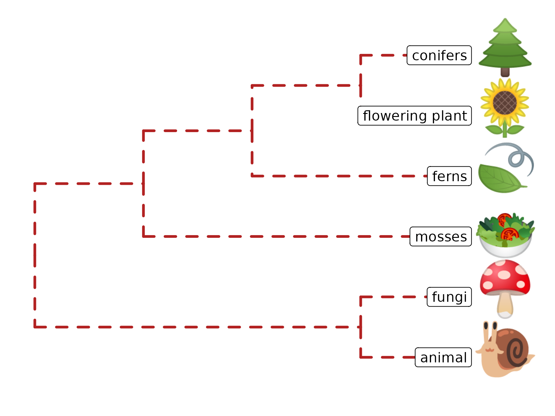

FIGURE 8.5: Parsing label as emoji. Text (e.g., node or tip labels) can be parsed as emoji.

Note that the output may depend on what emoji fonts are installed in your system¹⁷.

With ggtree, it is easy to generate phylomoji. The emoji is treated as text, like ‘abc’. We can use emojis to label taxa, clade, color and rotate emoji with any given color and angle. This functionality is internally supported by the emojifont package.

8.4.1 Emoji in circular/fan layout tree

It also works with circular and fan layouts as demonstrated in Figure 8.6.

p <- ggtree(tree, layout = "circular", size=1) +  
  geom_tiplab(parse="emoji", size=10, vjust=.25)
print(p)

## fan layout  
p2 <- open_tree(p, angle=200) 
print(p2)

p2 %>% rotate_tree(-90)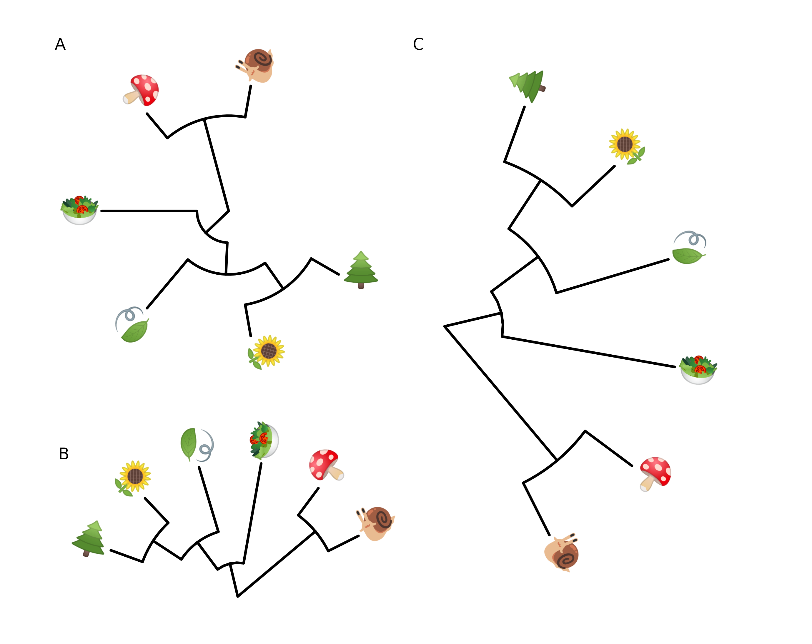

FIGURE 8.6: Phylomoji in cirular and fan layouts.

Another example using ggtree and emojifont to produce phylogeny of plant emojis can be found in a scientific article (Escudero & Wendel, 2020).

8.4.2 Emoji to label clades

Parsing clade labels as emojis is also supported in the geom_cladelab() layer. For example, in a phylogenetic tree of influenza viruses, we can use emojis to label clades to represent host species similar to Figure 8.7.

set.seed(123)
tr <- rtree(30)

dat <- data.frame(
           node = c(41, 53, 48),
           name = c("chicken", "duck", "family")
       )

p <- ggtree(tr) + 
     xlim(NA, 5.2) +
     geom_cladelab(
         data = dat,
         mapping = aes(
             node = node, 
             label = name, 
             color = name
         ),
         parse = "emoji",
         fontsize = 12,
         align = TRUE,
         show.legend = FALSE
     ) +
     scale_color_manual(
         values = c(
             chicken="firebrick", 
             duck="steelblue", 
             family = "darkkhaki"
         )
     )
p

FIGURE 8.7: Emoji to label clades.

8.4.3 Apple Color Emoji

Although R’s graphical devices don’t support AppleColorEmoji font on MacOS, it’s still possible to use it. We can export the plot to a svg file and render it in Safari (Figure 8.8).

library(ggtree)
tree_text <- paste0("(((((cow, (whale, dolphin)), (pig2, boar)),",
                    "camel), fish), seedling);")
x <- read.tree(text=tree_text)
library(ggimage)
p <-  ggtree(x, size=2) + geom_tiplab(size=20, parse='emoji') +
    xlim(NA, 7) + ylim(NA, 8.5) 

svglite::svglite("emoji.svg", width = 10, height = 7)
print(p)
dev.off()

# or use `grid.export()` 
# ps = gridSVG::grid.export("emoji.svg", addClass=T)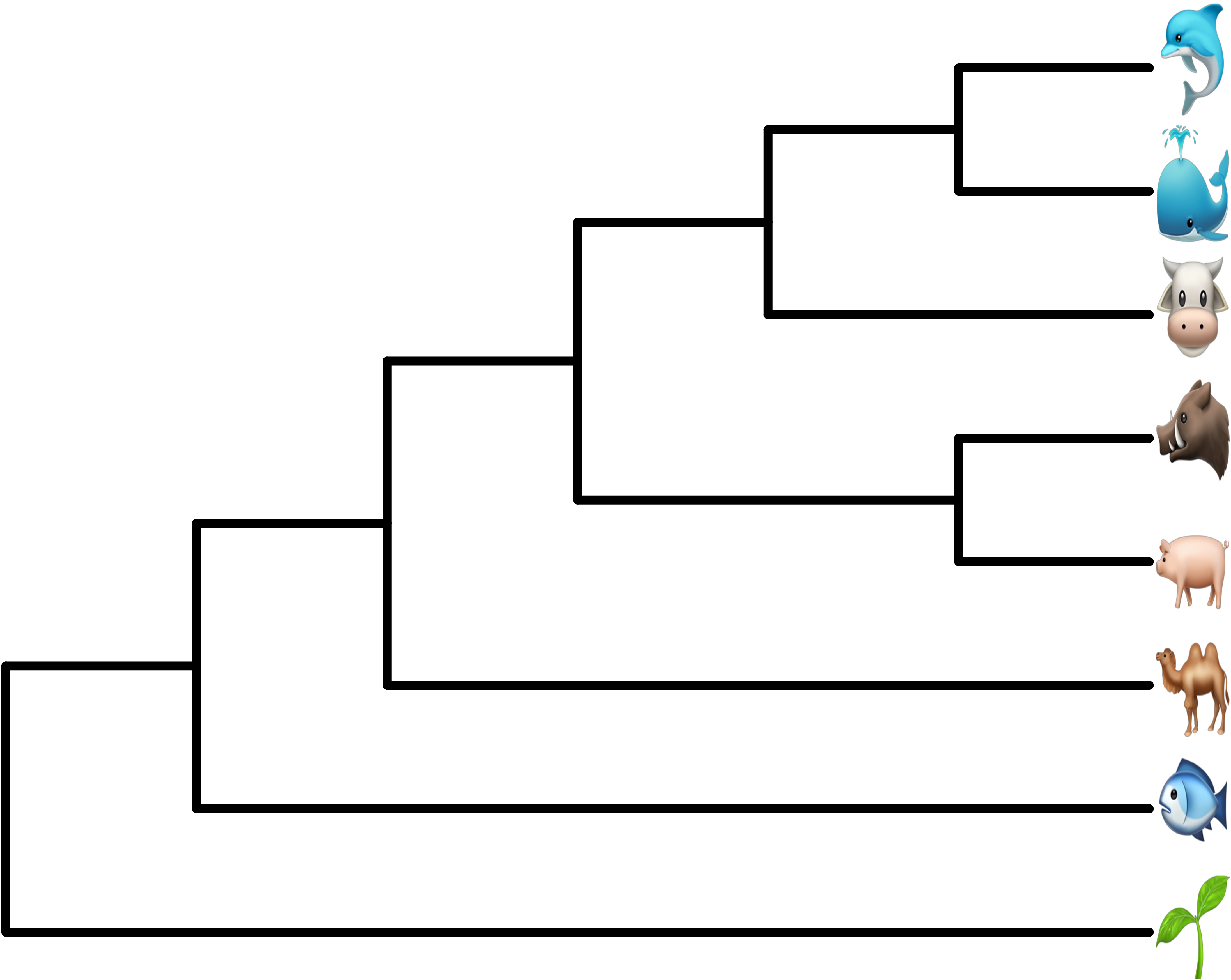

FIGURE 8.8: Use Apple Color Emoji in ggtree. The tip labels were parsed as emojis using AppleColorEmoji font in Safari.

8.4.4 Phylomoji in ASCII art

Producing phylomoji as an ASCII art is also possible. Users can refer to Appendix D for details.

8.5 Summary

The ggtree supports parsing labels, including tip labels, internal node labels, and clade labels, as images, math expression, and emoji, in case the labels can be parsed as image file names, plotmath expression, or emoji names, respectively. It can be fun, but it’s also very useful for scientific research. The use of images on phylogenetic trees can help to present species-related characteristics, including morphological, anatomical, and even macromolecular structures. Moreover, ggtree supports summarizing statistical inferences (e.g., biogeographic range reconstruction and posterior distribution) or associated data of the nodes as subplots to be displayed on a phylogenetic tree.