4 Phylogenetic Tree Visualization

4.1 Introduction

There are many software packages and web tools that are designed for displaying phylogenetic trees, such as TreeView (Page, 2002), FigTree, TreeDyn (Chevenet et al., 2006), Dendroscope (Huson & Scornavacca, 2012), EvolView (He et al., 2016), and iTOL (Letunic & Bork, 2007), etc. Only a few of them, such as FigTree, TreeDyn and iTOL, allow users to annotate the trees with colored branches, highlighted clades with tree features. However, their pre-defined annotating functions are usually limited to some specific phylogenetic data. As phylogenetic trees are becoming more widely used in multidisciplinary studies, there is an increasing need to incorporate various types of phylogenetic covariates and other associated data from different sources into the trees for visualizations and further analyses. For instance, the influenza virus has a wide host range, diverse and dynamic genotypes, and characteristic transmission behaviors that are mostly associated with the virus’s evolution and essentially among themselves. Therefore, in addition to standalone applications that focus on each of the specific analysis and data types, researchers studying molecular evolution need a robust and programmable platform that allows the high levels of integration and visualization of many of these different aspects of data (raw or from other primary analyses) over the phylogenetic trees to identify their associations and patterns.

To fill this gap, we developed ggtree (Yu et al., 2017), a package for the R programming language (R Core Team, 2016) released under the Bioconductor project (Gentleman et al., 2004). The ggtree is built to work with treedata objects (see Chapters 1 and 9), and display tree graphics with the ggplot2 package (Wickham, 2016) that was based on the grammar of graphics (Wilkinson et al., 2005).

The R language is increasingly used in phylogenetics. However, a comprehensive package, designed for viewing and annotating phylogenetic trees, particularly with complex data integration, is not yet available. Most of the R packages in phylogenetics focus on specific statistical analyses rather than viewing and annotating the trees with more generalized phylogeny-associated data. Some packages, including ape (Paradis et al., 2004) and phytools (Revell, 2012), which are capable of displaying and annotating trees, are developed using the base graphics system of R. In particular, ape is one of the fundamental packages for phylogenetic analysis and data processing. However, the base graphics system is relatively difficult to extend and limits the complexity of the tree figure to be displayed. OutbreakTools (Jombart et al., 2014) and phyloseq (McMurdie & Holmes, 2013) extended ggplot2 to plot phylogenetic trees. The ggplot2 system of graphics allows rapid customization and exploration of design solutions. However, these packages were designed for epidemiology and microbiome data respectively and did not aim to provide a general solution for tree visualization and annotation. The ggtree package also inherits versatile properties of ggplot2, and more importantly allows constructing complex tree figures by freely combining multiple layers of annotations (see also Chapter 5) using the tree associated data imported from different sources (see detailed in Chapter 1 and (Wang et al., 2020)).

4.2 Visualizing Phylogenetic Tree with ggtree

The ggtree package (Yu et al., 2017) is designed for annotating phylogenetic trees with their associated data of different types and from various sources. These data could come from users or analysis programs and might include evolutionary rates, ancestral sequences, etc. that are associated with the taxa from real samples, or with the internal nodes representing hypothetic ancestor strain/species, or with the tree branches indicating evolutionary time courses (Wang et al., 2020). For instance, the data could be the geographic positions of the sampled avian influenza viruses (informed by the survey locations) and the ancestral nodes (by phylogeographic inference) in the viral gene tree (Lam et al., 2012).

The ggtree supports ggplot2’s graphical language, which allows a high level of customization, is intuitive and flexible. Notably, ggplot2 itself does not provide low-level geometric objects or other support for tree-like structures, and hence ggtree is a useful extension in that regard. Even though the other two phylogenetics-related R packages, OutbreakTools, and phyloseq, are developed based on ggplot2, the most valuable part of the ggplot2 syntax - adding layers of annotations - is not supported in these packages. For example, if we have plotted a tree without taxa labels, OutbreakTools and phyloseq provide no easy way for general R users, who have little knowledge about the infrastructures of these packages, to add a layer of taxa labels. The ggtree extends ggplot2 to support tree objects by implementing a geometric layer, geom_tree(), to support visualizing tree structure. In ggtree, viewing a phylogenetic tree is relatively easy, via the command ggplot(tree_object) + geom_tree() + theme_tree() or ggtree(tree_object) for short. Layers of annotations can be added one-by-one via the + operator. To facilitate tree visualization, ggtree provides several geometric layers, including geom_treescale() for adding legend of tree branch scale (genetic distance, divergence time, etc.), geom_range() for displaying uncertainty of branch lengths (confidence interval or range, etc.), geom_tiplab() for adding taxa label, geom_tippoint() and geom_nodepoint() for adding symbols of tips and internal nodes, geom_hilight() for highlighting clades with rectangle, and geom_cladelab() for annotating selected clades with bar and text label, etc.. A full list of geometric layers provided by ggtree is summarized in Table 5.1.

To view a phylogenetic tree, we first need to parse the tree file into R. The treeio package is able to parse diverse annotation data from different software outputs into S4 phylogenetic data objects (see also Chapter 1). The ggtree package mainly utilizes these S4 objects to display and annotate the tree. Other R packages defined S3/S4 classes to store phylogenetic trees with domain-specific associated data, including phylo4 and phylo4d defined in the phylobase package, obkdata defined in the OutbreakTools package, and phyloseq defined in the phyloseq package, etc. All these tree objects are also supported in ggtree and their specific annotation data can be used to annotate the tree directly in ggtree (see also Chapter 9). Such compatibility of ggtree facilitates the integration of data and analysis results. In addition, ggtree also supports other tree-like structures, including dendrogram and tree graphs.

4.2.1 Basic Tree Visualization

The ggtree package extends ggplot2 (Wickham, 2016) package to support viewing a phylogenetic tree. It implements geom_tree() layer for displaying a phylogenetic tree, as shown below in Figure 4.1A.

library("treeio")
library("ggtree")

nwk <- system.file("extdata", "sample.nwk", package="treeio")
tree <- read.tree(nwk)

ggplot(tree, aes(x, y)) + geom_tree() + theme_tree()

The function, ggtree(), was implemented as a shortcut to visualize a tree, and it works exactly the same as shown above.

The ggtree package takes all the advantages of ggplot2. For example, we can change the color, size, and type of the lines as we do with ggplot2 (Figure 4.1B).

ggtree(tree, color="firebrick", size=2, linetype="dotted")

By default, the tree is viewed in ladderize form, user can set the parameter ladderize = FALSE to disable it (Figure 4.1C, see also FAQ A.5).

ggtree(tree, ladderize=FALSE)

The branch.length is used to scale the edge, user can set the parameter branch.length = "none" to only view the tree topology (cladogram, Figure 4.1D) or other numerical variables to scale the tree (e.g., d_N/d_S, see also in Chapter 5).

ggtree(tree, branch.length="none")

FIGURE 4.1: Basic tree visualization. Default ggtree output with ladderized effect (A), non-variable setting (e.g., color, size, line type) (B), non-ladderized tree (C), cladogram that only displays tree topology without branch length information (D).

4.2.2 Layouts of a phylogenetic tree

Viewing phylogenetic with ggtree is quite simple, just pass the tree object to the ggtree() function. We have developed several types of layouts for tree presentation (Figure 4.2), including rectangular (by default), roundrect (rounded rectangular), ellipse, slanted, circular, fan, unrooted (equal angle and daylight methods), time-scaled, and two-dimensional layouts.

Here are examples of visualizing a tree with different layouts:

library(ggtree)
set.seed(2017-02-16)
tree <- rtree(50)
ggtree(tree)
ggtree(tree, layout="roundrect")
ggtree(tree, layout="slanted")
ggtree(tree, layout="ellipse")
ggtree(tree, layout="circular")
ggtree(tree, layout="fan", open.angle=120)
ggtree(tree, layout="equal_angle")
ggtree(tree, layout="daylight")
ggtree(tree, branch.length='none')
ggtree(tree, layout="ellipse", branch.length="none")
ggtree(tree, branch.length='none', layout='circular')
ggtree(tree, layout="daylight", branch.length = 'none')

FIGURE 4.2: Tree layouts. Phylogram: rectangular layout (A), rounded rectangular layout (B), slanted layout (C), ellipse layout (D), circular layout (E), and fan layout (F). Unrooted: equal-angle method (G) and daylight method (H). Cladogram: rectangular layout (I), ellipse (J), circular layout (K), and unrooted layout (L). Slanted and fan layouts for cladogram are also supported.

Other possible layouts that can be drawn by modifying scales/coordination (Figure 4.3).

ggtree(tree) + scale_x_reverse()
ggtree(tree) + coord_flip()
ggtree(tree) + layout_dendrogram()
ggplotify::as.ggplot(ggtree(tree), angle=-30, scale=.9)
ggtree(tree, layout='slanted') + coord_flip()
ggtree(tree, layout='slanted', branch.length='none') + layout_dendrogram()
ggtree(tree, layout='circular') + xlim(-10, NA)
ggtree(tree) + layout_inward_circular()
ggtree(tree) + layout_inward_circular(xlim=15)

FIGURE 4.3: Derived Tree layouts. right-to-left rectangular layout (A), bottom-up rectangular layout (B), top-down rectangular layout (Dendrogram) (C), rotated rectangular layout (D), bottom-up slanted layout (E), top-down slanted layout (Cladogram) (F), circular layout (G), circular inward layout (H and I).

Phylogram. Layouts of rectangular, roundrect, slanted, ellipse, circular, and fan are supported to visualize phylogram (by default, with branch length scaled) as demonstrated in Figures 4.2A-F.

Unrooted layout. Unrooted (also called ‘radial’) layout is supported by equal-angle and daylight algorithms; users can specify unrooted layout algorithm by passing “equal_angle” or “daylight” to layout parameter to visualize the tree. The equal-angle method was proposed by Christopher Meacham in PLOTREE, which was incorporated in PHYLIP (Retief, 2000). This method starts from the root of the tree and allocates arcs of angle to each subtree proportional to the number of tips in it. It iterates from root to tips and subdivides the angle allocated to a subtree into angles for its dependent subtrees. This method is fast and was implemented in many software packages. As shown in Figure 4.2G, the equal angle method has a drawback that tips tend to be clustered together, which will leave many spaces unused. The daylight method starts from an initial tree built by equal angle and iteratively improves it by successively going to each interior node and swinging subtrees so that the arcs of “daylight” are equal (Figure 4.2H). This method was firstly implemented in PAUP* (Wilgenbusch & Swofford, 2003).

Cladogram. To visualize a cladogram that is without branch length scaling and only displays the tree structure, branch.length is set to “none” and it works for all types of layouts (Figures 4.2I-L).

Timescaled layout. For a timescaled tree, the most recent sampling date must be specified via the mrsd parameter, and ggtree() will scale the tree by sampling (tip) and divergence (internal node) time, and a timescale axis will be displayed under the tree by default. Users can use the deeptime package to add geologic timescale (e.g., periods and eras) to a ggtree() plot.

beast_file <- system.file("examples/MCC_FluA_H3.tree", 
                          package="ggtree")
beast_tree <- read.beast(beast_file)
ggtree(beast_tree, mrsd="2013-01-01") + theme_tree2()

FIGURE 4.4: Timescaled layout. The x-axis is the timescale (in units of the year). The divergence time in this example was inferred by BEAST using the molecular clock model.

Two-dimensional tree layout. A two-dimensional tree is a projection of the phylogenetic tree in a space defined by the associated phenotype (numerical or categorical trait, on the y-axis) and tree branch scale (e.g., evolutionary distance, divergent time, on the x-axis). The phenotype can be a measure of certain biological characteristics of the taxa and hypothetical ancestors in the tree. This layout is useful to track the virus phenotypes or other behaviors (y-axis) changing with the virus evolution (x-axis). In fact, the analysis of phenotypes or genotypes over evolutionary time have been widely used for study of influenza virus evolution (Neher et al., 2016), though such analysis diagrams are not tree-like, i.e., no connection between data points, unlike our two-dimensional tree layout that connects data points with the corresponding tree branches. Therefore, this new layout we provided will make such data analysis easier and more scalable for large sequence datasets.

In this example, we used the previous timescaled tree of H3 human and swine influenza viruses (Figure 4.4; data published in (Liang et al., 2014)) and scaled the y-axis based on the predicted N-linked glycosylation sites (NLG) for each of the taxon and ancestral sequences of hemagglutinin proteins. The NLG sites were predicted using the NetNGlyc 1.0 Server. To scale the y-axis, the parameter yscale in the ggtree() function is set to a numerical or categorical variable. If yscale is a categorical variable as in this example, users should specify how the categories are to be mapped to numerical values via the yscale_mapping variables.

NAG_file <- system.file("examples/NAG_inHA1.txt", package="ggtree")

NAG.df <- read.table(NAG_file, sep="\t", header=FALSE, 
                     stringsAsFactors = FALSE)
NAG <- NAG.df[,2]
names(NAG) <- NAG.df[,1]

## separate the tree by host species
tip <- as.phylo(beast_tree)$tip.label
beast_tree <- groupOTU(beast_tree, tip[grep("Swine", tip)], 
                       group_name = "host")

p <- ggtree(beast_tree, aes(color=host), mrsd="2013-01-01", 
            yscale = "label", yscale_mapping = NAG) + 
  theme_classic() + theme(legend.position='none') +
  scale_color_manual(values=c("blue", "red"), 
                     labels=c("human", "swine")) +
  ylab("Number of predicted N-linked glycosylation sites")

## (optional) add more annotations to help interpretation
p + geom_nodepoint(color="grey", size=3, alpha=.8) +
  geom_rootpoint(color="black", size=3) +
  geom_tippoint(size=3, alpha=.5) + 
  annotate("point", 1992, 5.6, size=3, color="black") +
  annotate("point", 1992, 5.4, size=3, color="grey") +
  annotate("point", 1991.6, 5.2, size=3, color="blue") +
  annotate("point", 1992, 5.2, size=3, color="red") + 
  annotate("text", 1992.3, 5.6, hjust=0, size=4, label="Root node") +
  annotate("text", 1992.3, 5.4, hjust=0, size=4, 
           label="Internal nodes") +
  annotate("text", 1992.3, 5.2, hjust=0, size=4,
           label="Tip nodes (blue: human; red: swine)")

FIGURE 4.5: Two-dimensional tree layout. The trunk and other branches are highlighted in red (for swine) and blue (for humans). The x-axis is scaled to the branch length (in units of year) of the timescaled tree. The y-axis is scaled to the node attribute variable, in this case, the number of predicted N-linked glycosylation sites (NLG) on the hemagglutinin protein. Colored circles indicate the different types of tree nodes. Note that nodes assigned the same x- (temporal) and y- (NLG) coordinates are superimposed in this representation and appear as one node, which is shaded based on the colors of all the nodes at that point.

As shown in Figure 4.5, a two-dimensional tree is good at visualizing the change of phenotype over the evolution in the phylogenetic tree. In this example, it is shown that the H3 gene of the human influenza A virus maintained a high level of N-linked glycosylation sites (n=8 to 9) over the last two decades and dropped significantly to 5 or 6 in a separate viral lineage transmitted to swine populations and established there. It was indeed hypothesized that the human influenza virus with a high level of glycosylation on the viral hemagglutinin protein provides a better shielding effect to protect the antigenic sites from exposure to the herd immunity, and thus has a selective advantage in human populations that maintain a high level of herd immunity against the circulating human influenza virus strains. For the viral lineage that newly jumped across the species barrier and transmitted to the swine population, the shielding effect of the high-level surface glycan oppositely imposes selective disadvantage because the receptor-binding domain may also be shielded which greatly affects the viral fitness of the lineage that newly adapted to a new host species. Another example of a two-dimensional tree can be found in Figure 4.12.

4.3 Displaying Tree Components

4.3.1 Displaying treescale (evolution distance)

To show treescale, the user can use geom_treescale() layer (Figures 4.6A-C).

ggtree(tree) + geom_treescale()

geom_treescale() supports the following parameters:

• x and y for treescale position
• width for the length of the treescale
• fontsize for the size of the text
• linesize for the size of the line
• offset for relative position of the line and the text
• color for color of the treescale

ggtree(tree) + geom_treescale(x=0, y=45, width=1, color='red')
ggtree(tree) + geom_treescale(fontsize=6, linesize=2, offset=1)

We can also use theme_tree2() to display the treescale by adding x axis (Figure 4.6D).

ggtree(tree) + theme_tree2()

FIGURE 4.6: Display treescale. geom_treescale() automatically add a scale bar for evolutionary distance (A). Users can modify the color, width, and position of the scale (B) as well as the size of the scale bar and text and their relative position (C). Another possible solution is to enable the x-axis which is useful for the timescaled tree (D).

Treescale is not restricted to evolution distance, treeio can rescale the tree with other numerical variables (details described in session 2.4), and ggtree allows users to specify a numerical variable to serve as branch length for visualization (details described in session 4.3).

4.3.2 Displaying nodes/tips

Showing all the internal nodes and tips in the tree can be done by adding a layer of points using geom_nodepoint(), geom_tippoint(), or geom_point() (Figure 4.7).

ggtree(tree) + 
    geom_point(aes(shape=isTip, color=isTip), size=3)

p <- ggtree(tree) + 
    geom_nodepoint(color="#b5e521", alpha=1/4, size=10) 
p + geom_tippoint(color="#FDAC4F", shape=8, size=3)

FIGURE 4.7: Display external and internal nodes. geom_point() automatically add symbolic points of all nodes (A). geom_nodepoint() adds symbolic points for internal nodes and geom_tippoint() adds symbolic points for external nodes (B).

4.3.3 Displaying labels

Users can use geom_text() or geom_label() to display the node (if available) and tip labels simultaneously or geom_tiplab() to only display tip labels (Figure 4.8A).

p + geom_tiplab(size=3, color="purple")

The geom_tiplab() layer not only supports using text or label geom to display labels, but it also supports image geom to label tip with image files (see Chapter 7). A corresponding geom, geom_nodelab() is also provided for displaying node labels.

For circular and unrooted layouts, ggtree supports rotating node labels according to the angles of the branches (Figure 4.8B).

ggtree(tree, layout="circular") + geom_tiplab(aes(angle=angle), color='blue')

For long tip labels, the label may be truncated. There are several ways to solve this issue (see FAQ: Tip label truncated). Another solution to solve this issue is to display tip labels as y-axis labels (Figure 4.8C). However, it only works for rectangular and dendrogram layouts and users need to use theme() to adjust tip labels in this case.

ggtree(tree) + geom_tiplab(as_ylab=TRUE, color='firebrick')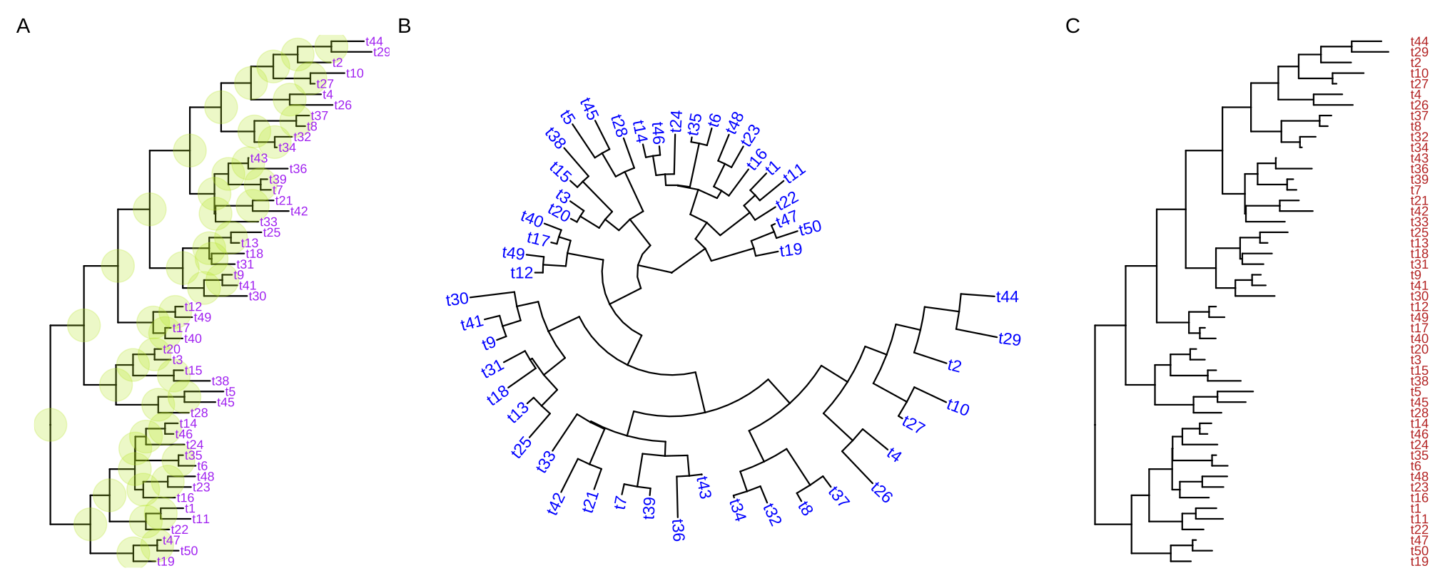

FIGURE 4.8: Display tip labels. geom_tiplab() supports displaying tip labels (A). For the circular, fan, or unrooted tree layouts, the labels can be rotated to fit the angle of the branches (B). For dendrogram/rectangular layout, tip labels can be displayed as y-axis labels (C).

By default, the positions to display text are based on the node positions; we can change them to be based on the middle of the branch/edge (by setting aes(x = branch)), which is very useful when annotating transition from the parent node to the child node.

4.3.4 Displaying root-edge

The ggtree() doesn’t plot the root-edge by default. Users can use geom_rootedge() to automatically display the root-edge (Figure 4.9A). If there is no root edge information, geom_rootedge() will display nothing by default (Figure 4.9B). Users can set the root-edge to the tree (Figure 4.9C) or specify rootedge in geom_rootedge() (Figure 4.9D). A long root length is useful to increase readability of the circular tree (see also FAQ: Enlarge center space).

## with root-edge = 1
tree1 <- read.tree(text='((A:1,B:2):3,C:2):1;')
ggtree(tree1) + geom_tiplab() + geom_rootedge()

## without root-edge
tree2 <- read.tree(text='((A:1,B:2):3,C:2);')
ggtree(tree2) + geom_tiplab() + geom_rootedge()

## setting root-edge
tree2$root.edge <- 2
ggtree(tree2) + geom_tiplab() + geom_rootedge()

## specify the length of root edge for just plotting
## this will ignore tree$root.edge
ggtree(tree2) + geom_tiplab() + geom_rootedge(rootedge = 3)

FIGURE 4.9: Display root-edge. geom_rootedge() supports displaying root-edge if the root edge was presented (A). It shows nothing if there is no root-edge (B). In this case, users can manually set the root edge for the tree (C) or just specify the length of the root for plotting (D).

4.3.5 Color tree

In ggtree (Yu et al., 2018), coloring phylogenetic tree is easy, by using aes(color=VAR) to map the color of the tree based on a specific variable (both numerical and categorical variables are supported, see Figure 4.10).

ggtree(beast_tree, aes(color=rate)) +
    scale_color_continuous(low='darkgreen', high='red') +
    theme(legend.position="right")

FIGURE 4.10: Color tree by continuous or discrete feature. Edges are colored by values associated with the child nodes.

Users can use any feature (if available), including clade posterior and d_N/d_S, etc., to scale the color of the tree. If the feature is a continuous numerical value, ggtree provides a continuous parameter to support plotting continuous state transition in edges. Here, we use an example⁹ to demonstrate this functionality (Figure 4.11A). If you want to add a thin black border in tree branches, you can place a tree with black and slightly thicker branches below your tree to emulate edge outlines as demonstrated in Figure 4.11B.

library(ggtree)
library(treeio)
library(tidytree)
library(ggplot2)
library(TDbook)
## ref: http://www.phytools.org/eqg2015/asr.html
##
## load `tree_anole` and `df_svl` from 'TDbook'
svl <- as.matrix(df_svl)[,1]
fit <- phytools::fastAnc(tree_anole, svl, vars=TRUE, CI=TRUE)

td <- data.frame(node = nodeid(tree_anole, names(svl)),
               trait = svl)
nd <- data.frame(node = names(fit$ace), trait = fit$ace)

d <- rbind(td, nd)
d$node <- as.numeric(d$node)
tree <- full_join(tree_anole, d, by = 'node')

p1 <- ggtree(tree, aes(color=trait), layout = 'circular', 
        ladderize = FALSE, continuous = 'colour', size=2) +
    scale_color_gradientn(colours=c("red", 'orange', 'green', 'cyan', 'blue')) +
    geom_tiplab(hjust = -.1) + 
    xlim(0, 1.2) + 
    theme(legend.position = c(.05, .85)) 

p2 <- ggtree(tree, layout='circular', ladderize = FALSE, size=2.8) + 
    geom_tree(aes(color=trait), continuous = 'colour', size=2) +  
    scale_color_gradientn(colours=c("red", 'orange', 'green', 'cyan', 'blue')) +
    geom_tiplab(aes(color=trait), hjust = -.1) + 
    xlim(0, 1.2) + 
    theme(legend.position = c(.05, .85)) 

plot_list(p1, p2, ncol=2, tag_levels="A")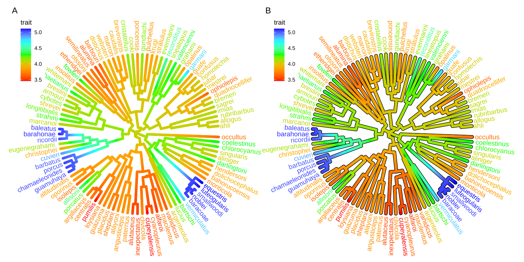    

FIGURE 4.11: Continuous state transition in edges. Edges are colored by the values from ancestral trait to offspring.

Besides, we can use a two-dimensional tree (as demonstrated in Figure 4.5) to visualize phenotype on the vertical dimension to create the phenogram Figure 4.12. We can use the ggrepel package to repel tip labels to avoid overlapping as demonstrated in Figure A.4.

ggtree(tree, aes(color=trait), continuous = 'colour', yscale = "trait") + 
    scale_color_viridis_c() + theme_minimal()

FIGURE 4.12: Phenogram. Projecting the tree into a space defined by time (or genetic distance) on the horizontal axis and phenotype on the vertical dimension.

4.3.6 Rescale tree

Most of the phylogenetic trees are scaled by evolutionary distance (substitution/site). In ggtree, users can rescale a phylogenetic tree by any numerical variable inferred by evolutionary analysis (e.g., d_N/d_S).

This example displays a time tree (Figure 4.13A) and the branches were rescaled by substitution rate inferred by BEAST (Figure 4.13B).

library("treeio")
beast_file <- system.file("examples/MCC_FluA_H3.tree", package="ggtree")
beast_tree <- read.beast(beast_file)
beast_tree

## 'treedata' S4 object that stored information
## of
##  '/home/ygc/R/library/ggtree/examples/MCC_FluA_H3.tree'.
## 
## ...@ phylo:
## 
## Phylogenetic tree with 76 tips and 75 internal nodes.
## 
## Tip labels:
##   A/Hokkaido/30-1-a/2013, A/New_York/334/2004,
## A/New_York/463/2005, A/New_York/452/1999,
## A/New_York/238/2005, A/New_York/523/1998, ...
## 
## Rooted; includes branch lengths.
## 
## with the following features available:
##   'height', 'height_0.95_HPD', 'height_median',
## 'height_range', 'length', 'length_0.95_HPD',
## 'length_median', 'length_range', 'posterior', 'rate',
## 'rate_0.95_HPD', 'rate_median', 'rate_range'.

p1 <- ggtree(beast_tree, mrsd='2013-01-01') + theme_tree2() +
    labs(caption="Divergence time")
p2 <- ggtree(beast_tree, branch.length='rate') + theme_tree2() +
    labs(caption="Substitution rate")

The following example draws a tree inferred by CodeML (Figure 4.13C), and the branches can be rescaled by using d_N/d_S values (Figure 4.13D).

mlcfile <- system.file("extdata/PAML_Codeml", "mlc", package="treeio")
mlc_tree <- read.codeml_mlc(mlcfile)
p3 <- ggtree(mlc_tree) + theme_tree2() +
    labs(caption="nucleotide substitutions per codon")
p4 <- ggtree(mlc_tree, branch.length='dN_vs_dS') + theme_tree2() +
    labs(caption="dN/dS tree")

FIGURE 4.13: Rescale tree branches. A time-scaled tree inferred by BEAST (A) and its branches were rescaled by substitution rate (B). A tree was inferred by CodeML (C) and the branches were rescaled by d_N/d_S values (D).

This provides a very convenient way to allow us to explore the relationship between tree associated data and tree structure through visualization. In addition to specifying branch.length in tree visualization, users can change branch length stored in tree object by using rescale_tree() function provided by the treeio package (Wang et al., 2020), and the following command will display a tree that is identical to Figure 4.13B. The rescale_tree() function was documented in session 2.4.

beast_tree2 <- rescale_tree(beast_tree, branch.length='rate')
ggtree(beast_tree2) + theme_tree2()

4.3.7 Modify components of a theme

The theme_tree() defined a totally blank canvas, while theme_tree2() adds phylogenetic distance (via x-axis). These two themes all accept a parameter of bgcolor that defined the background color. Users can use any theme components to the theme_tree() or theme_tree2() functions to modify them (Figure 4.14).

set.seed(2019)
x <- rtree(30)
ggtree(x, color="#0808E5", size=1) + theme_tree("#FEE4E9")
ggtree(x, color="orange", size=1) + theme_tree('grey30')

FIGURE 4.14: Three themes. All ggplot2 theme components can be modified, and all the ggplot2 themes can be applied to ggtree() output.

Users can also use an image file as the tree background, see example in Appendix B.

4.4 Visualize a List of Trees

The ggtree supports multiPhylo and treedataList objects and a list of trees can be viewed simultaneously. The trees will visualize one on top of another and can be plotted in different panels through facet_wrap() or facet_grid() functions (Figure 4.15).

## trees <- lapply(c(10, 20, 40), rtree)
## class(trees) <- "multiPhylo"
## ggtree(trees) + facet_wrap(~.id, scale="free") + geom_tiplab()

f <- system.file("extdata/r8s", "H3_r8s_output.log", package="treeio")
r8s <- read.r8s(f)
ggtree(r8s) + facet_wrap( ~.id, scale="free") + theme_tree2()

FIGURE 4.15: Visualizing multiPhylo object. The ggtree() function supports visualizing multiple trees stored in the multiPhylo or treedataList objects.

One hundred bootstrap trees can also be viewed simultaneously (Figure 4.16). This allows researchers to explore a large set of phylogenetic trees to find consensus and distinct trees. The consensus tree can be summarized via a density tree (Figure 4.18).

btrees <- read.tree(system.file("extdata/RAxML", 
                                "RAxML_bootstrap.H3", 
                                package="treeio")
                    )
ggtree(btrees) + facet_wrap(~.id, ncol=10)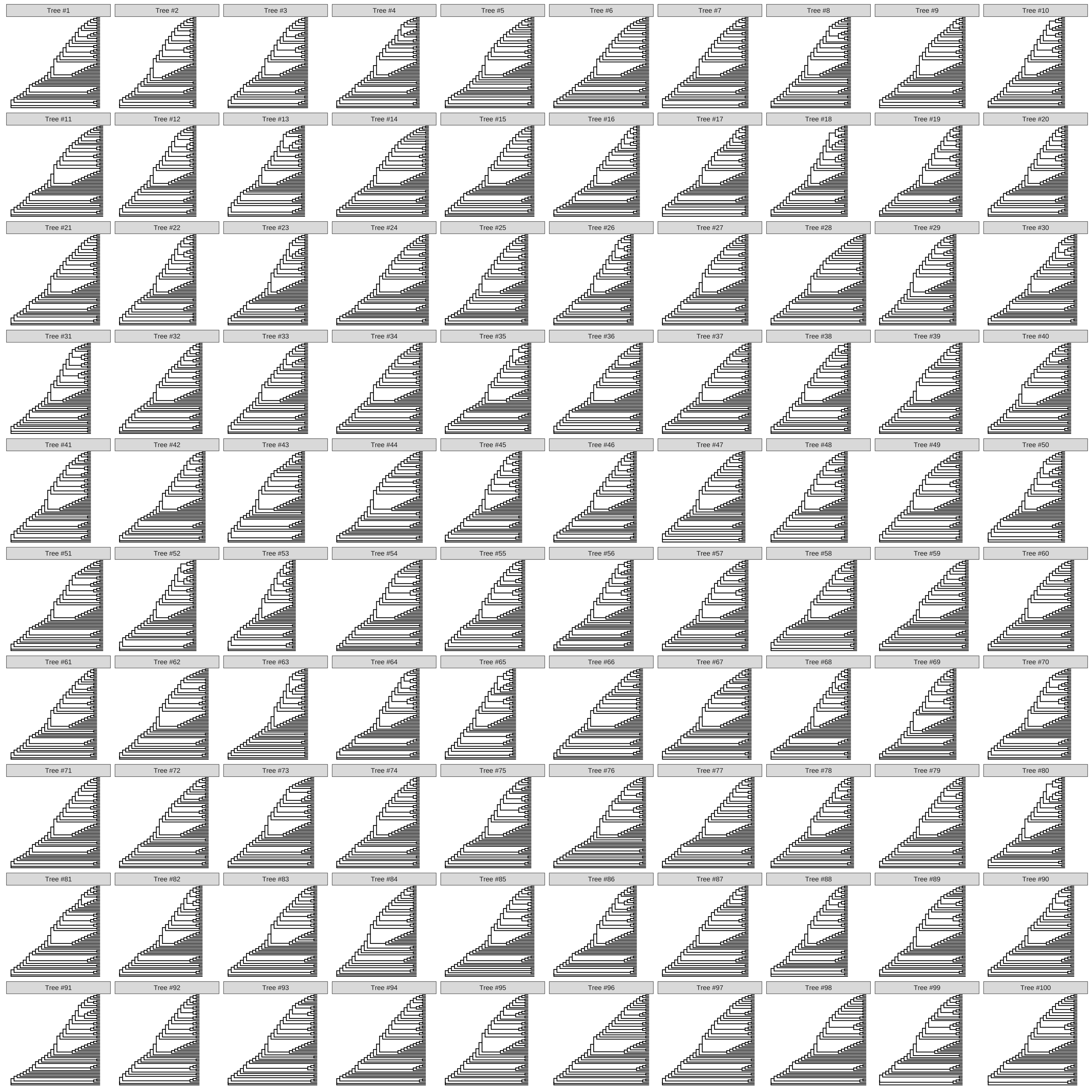

FIGURE 4.16: Visualizing one hundred bootstrap trees simultaneously.

4.4.1 Annotate one tree with values from different variables

To annotate one tree (the same tree) with the values from different variables, one can plot them separately and use patchwork or aplot to combine them side-by-side.

Another solution is to utilize the ability to plot a list of trees by ggtree, and then add annotation layers for the selected variable at a specific panel via the subset aesthetic mapping supported by ggtree or using the td_filter() as demonstrated in Figure 4.17. The .id is the conserved variable that is internally used to store the IDs of different trees.

set.seed(2020)
x <- rtree(30)
d <- data.frame(label=x$tip.label, var1=abs(rnorm(30)), var2=abs(rnorm(30)))
tree <- full_join(x, d, by='label')
trs <- list(TREE1 = tree, TREE2 = tree)
class(trs) <- 'treedataList'
ggtree(trs) + facet_wrap(~.id) + 
  geom_tippoint(aes(subset=.id == 'TREE1', colour=var1)) + 
  scale_colour_gradient(low='blue', high='red') +  
  ggnewscale::new_scale_colour()  + 
  geom_tippoint(aes(colour=var2), data=td_filter(.id == "TREE2")) + 
  scale_colour_viridis_c()

FIGURE 4.17: Annotate one tree with values from different variables. Using subset aesthetic mapping (as in TREE1 panel) or td_filter() (as in TREE2 panel) to filter variables to be displayed on the specific panel.

4.4.2 DensiTree

Another way to view the bootstrap trees is to merge them to form a density tree using ggdensitree() function (Figure 4.18). This will help us identify consensus and differences among a large set of trees. The trees will be stacked on top of each other and the structures of the trees will be rotated to ensure the consistency of the tip order. The tip order is determined by the tip.order parameter and by default (tip.order = 'mode') the tips are ordered by the most commonly seen topology. The user can pass in a character vector to specify the tip order, or pass in an integer, N, to order the tips by the order of the tips in the Nth tree. Passing mds to tip.order will order the tips based on MDS (Multidimensional Scaling) of the path length between the tips, or passing mds_dist will order the tips based on MDS of the distance between the tips.

ggdensitree(btrees, alpha=.3, colour='steelblue') + 
    geom_tiplab(size=3) + hexpand(.35)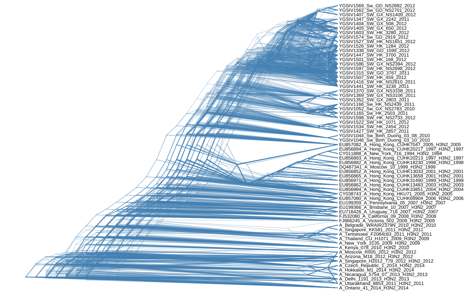

FIGURE 4.18: DensiTree. Trees are stacked on top of each other and the structures of the trees are rotated to ensure the consistency of the tip order.

4.5 Summary

Visualizing phylogenetic trees with ggtree is easy by using a single command ggtree(tree). The ggtree package provides several geometric layers to display tree components such as tip labels, symbolic points for both external and internal nodes, root-edge, etc. Associated data can be used to rescale branch lengths, color the tree, and be displayed on the tree. All these can be done by the ggplot2 grammar of graphic syntax, which makes it very easy to overlay layers and customize the tree graph (via ggplot2 themes and scales). The ggtree package also provides several layers that are specifically designed for tree annotation which will be introduced in Chapter 5. The ggtree package makes the presentation of trees and associated data extremely easy. Simple graphs are easy to generate, while complex graphs are simply superimposed layers and are also easy to generate.