5 Trajectory inference and RNA velocity

According to Wikipedia:

Trajectory inference or pseudotemporal ordering is a computational technique used in single-cell transcriptomics to determine the pattern of a dynamic process experienced by cells and then arrange cells based on their progression through the process.

It should be noted that all trajectory inference methods are based on the current transcriptional state and the distance symmetry between cells. That is to say, the distance from cell A to cell B is equal to the distance from cell B to cell A. Therefore, the direction of the inferred trajectory is either missing (requiring user specification) or unreliable (using default settings).

5.1 Slingshot: cell lineage and pseudotime inference

panc <- readRDS("data/pancreas_sub_sce.rds")

panc <- RunSlingshot(sce = panc, group = "SubCellType", reduction = "UMAP")

## Found more than one class "package_version" in cache; using the first, from namespace 'SeuratObject'

## Also defined by 'alabaster.base'

## Found more than one class "package_version" in cache; using the first, from namespace 'SeuratObject'

## Also defined by 'alabaster.base'

## Found more than one class "package_version" in cache; using the first, from namespace 'SeuratObject'

## Also defined by 'alabaster.base'

5.1.1 Lineage plot

p1 <- lineage_plot(panc, group = "SubCellType") + 
  sc_dim_geom_label(
    geom = shadowtext::geom_shadowtext,
    color='black', 
    bg.color='white'
  )

## Found more than one class "package_version" in cache; using the first, from namespace 'SeuratObject'

## Also defined by 'alabaster.base'

## Found more than one class "package_version" in cache; using the first, from namespace 'SeuratObject'

## Also defined by 'alabaster.base'

## displayed selected lineages
p2 <- lineage_plot(panc, group = "SubCellType", lineages = c("Lineage1", "Lineage2"))  + 
  sc_dim_geom_label(
    geom = shadowtext::geom_shadowtext,
    color='black', 
    bg.color='white'
  )

## Found more than one class "package_version" in cache; using the first, from namespace 'SeuratObject'
## Also defined by 'alabaster.base'

## Found more than one class "package_version" in cache; using the first, from namespace 'SeuratObject'

## Also defined by 'alabaster.base'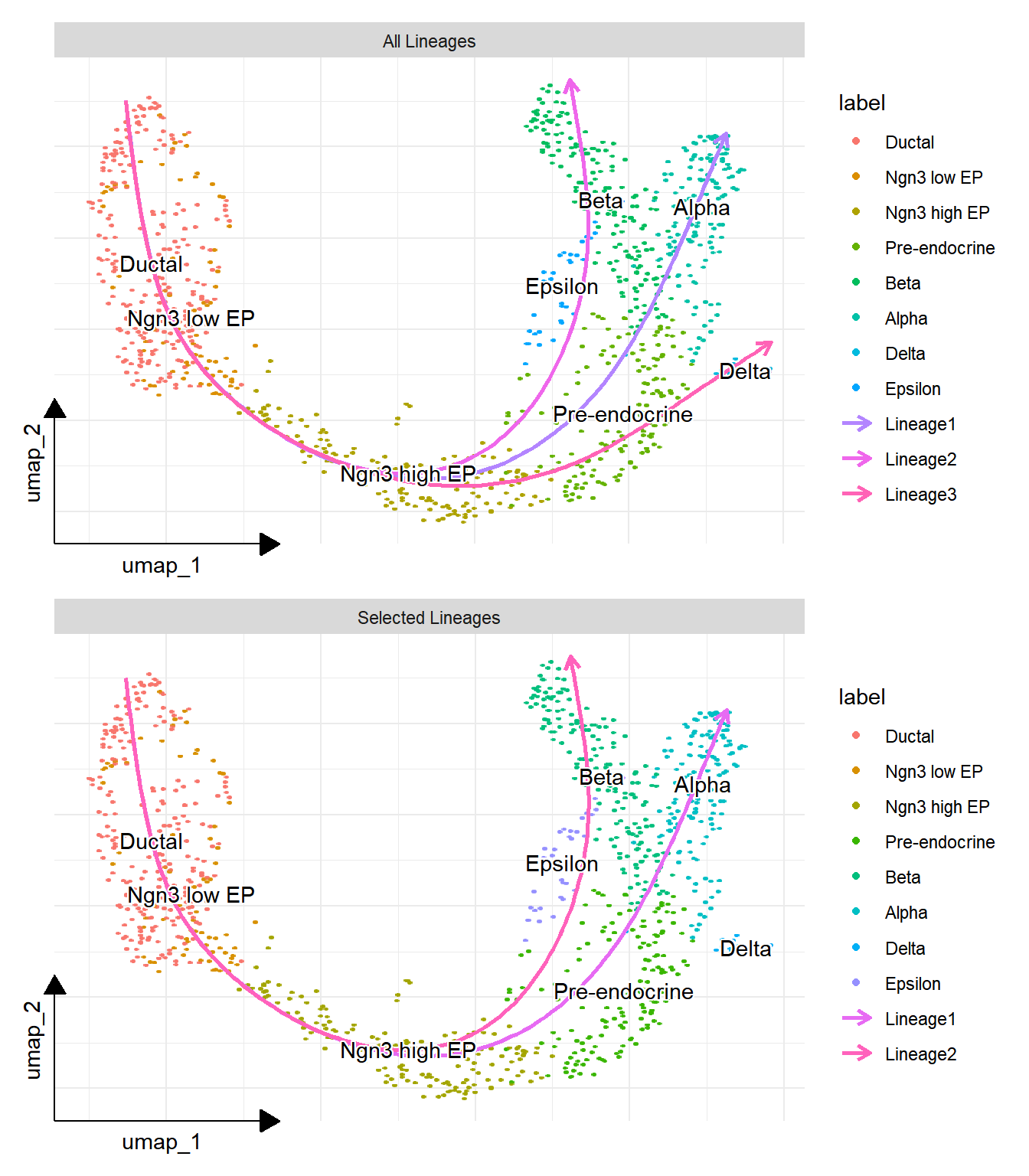

plot_list(`All Lineages` = p1, `Selected Lineages` = p2, ncol=1)

5.1.2 Pseudotime plot

pp1 <- pseudo_plot(panc, reduction = "UMAP", lineage = "Lineage1")

## Found more than one class "package_version" in cache; using the first, from namespace 'SeuratObject'

## Also defined by 'alabaster.base'

pp2 <- pseudo_plot(panc, reduction = "UMAP", lineage = "Lineage2")

## Found more than one class "package_version" in cache; using the first, from namespace 'SeuratObject'
## Also defined by 'alabaster.base'

pp_all <- pseudo_plot(panc, reduction = "UMAP")

## Found more than one class "package_version" in cache; using the first, from namespace 'SeuratObject'
## Also defined by 'alabaster.base'

plot_list(pp1, pp2, pp_all, design="AABB\nCCCC")

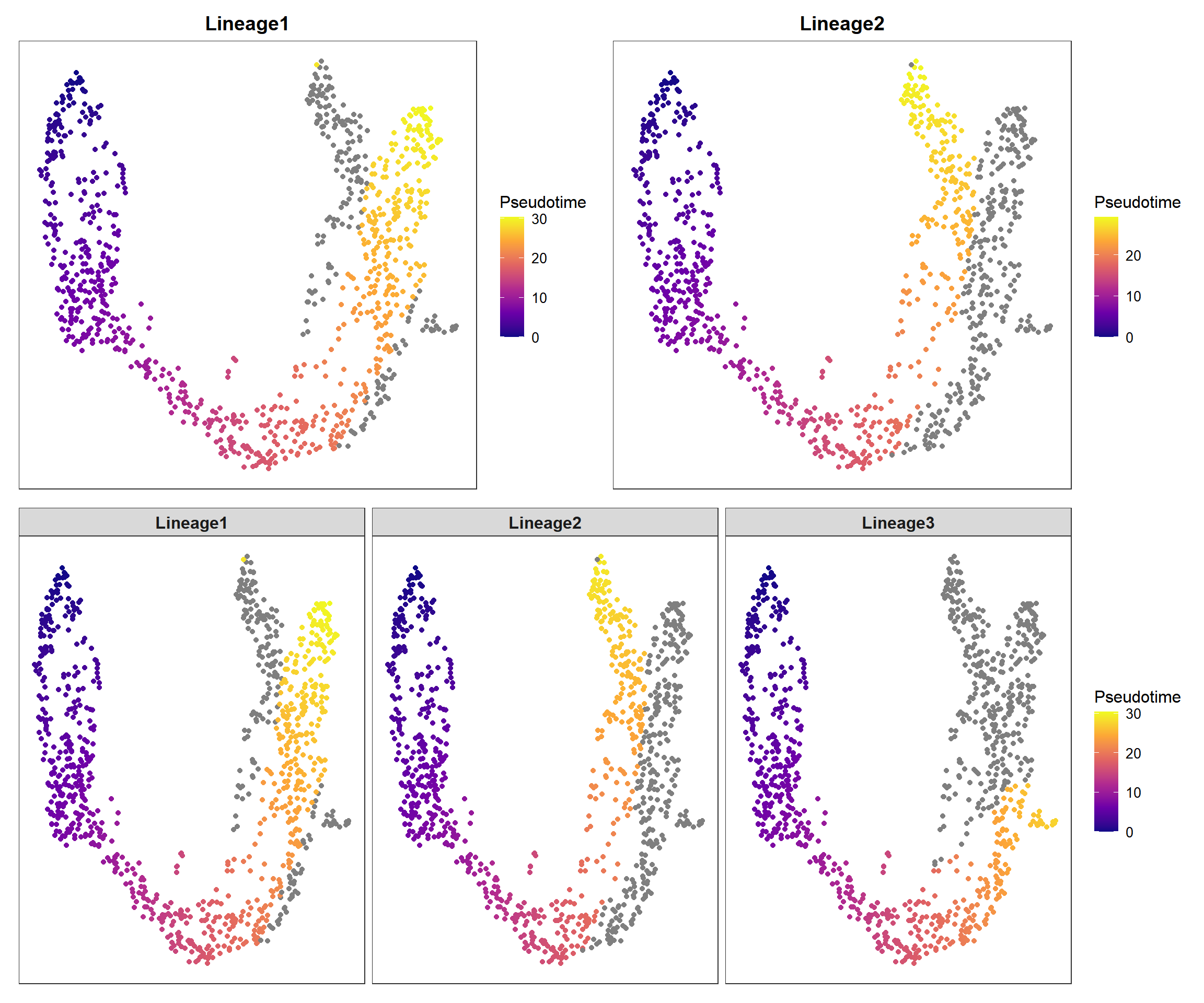
5.1.3 Expression trends in different cell trajectories

curve_genes <- c("Mrpl15", "Tram1", "Ncoa2")

## 默认选取smooth方法直接拟合得到的基因表达值结果来画图
p_curve <- genecurve_plot(panc, features = curve_genes, method = "smooth")

## 也可以用GAM计算预测的基因表达值来画图
p_curve1 <- genecurve_plot(panc, features = curve_genes, method = "gam")

plot_list(p_curve, p_curve1, ncol=1)

## `geom_smooth()` using method = 'loess' and formula = 'y ~
## x'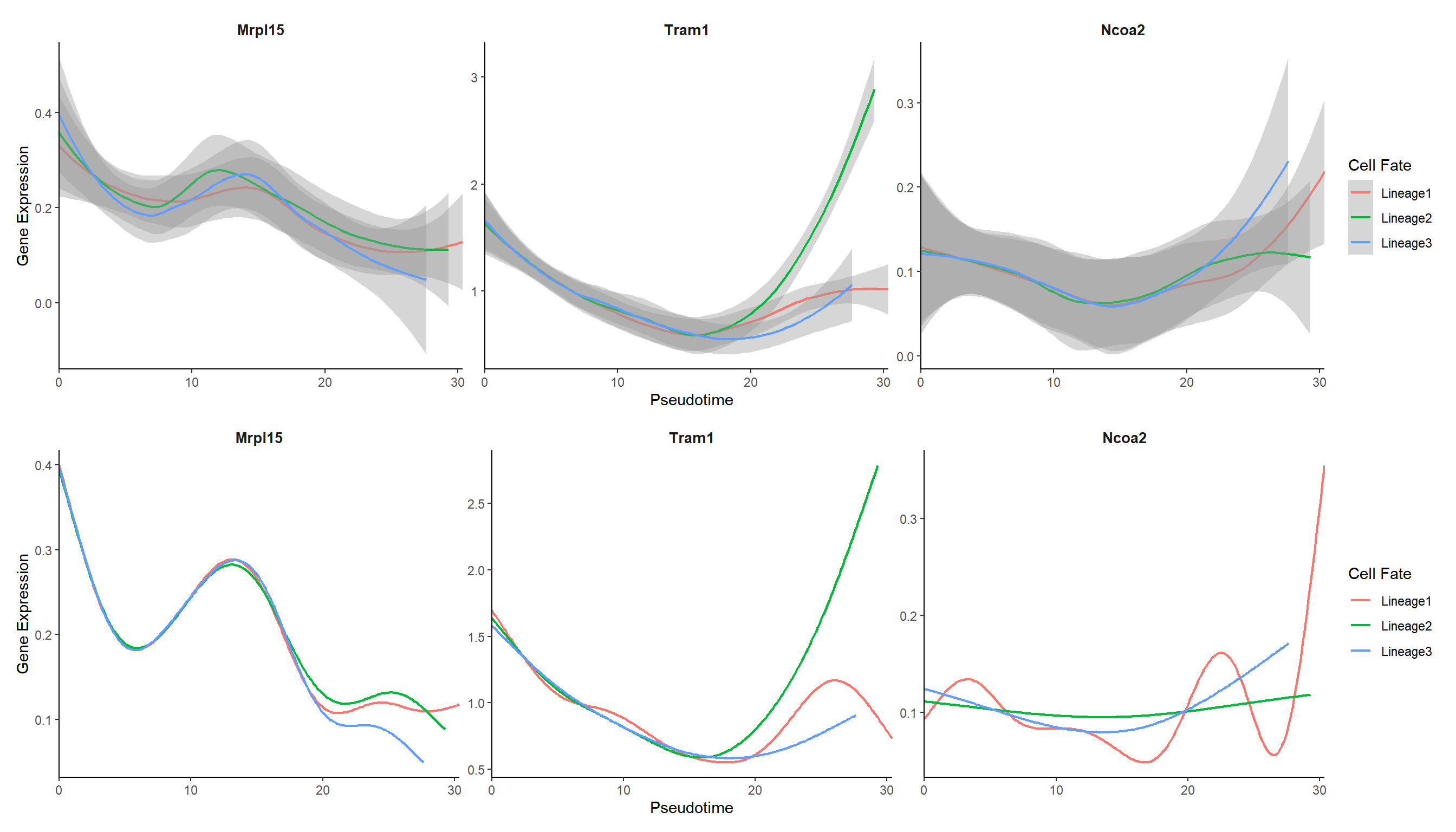

5.1.4 Heatmap

heatmap_genes <- head(unique(rownames(panc)), 10)

## 默认按照拟时间排序
hmp1 <- pseudo_heatmap(panc, features = heatmap_genes, lineage = "Lineage2")

## 可以手动对基因或细胞设置聚类(cluster = TRUE)，此时会打乱pseudotime的排序
hmp2 <- pseudo_heatmap(panc, features = heatmap_genes, lineage = "Lineage2", cluster_columns = TRUE)

## 对基因聚类
hmp3 <- pseudo_heatmap(panc, features = heatmap_genes, lineage = "Lineage2", cluster_rows = TRUE, sort = FALSE)

## 默认排序
hmp4 <- pseudo_heatmap(panc, features = heatmap_genes, lineage = "Lineage2", cluster_rows = FALSE, sort = TRUE)

## 组合起来看就能看到两个参数的设定对行顺序的影响
plot_list(hmp1, hmp2, hmp3, hmp4, ncol=1)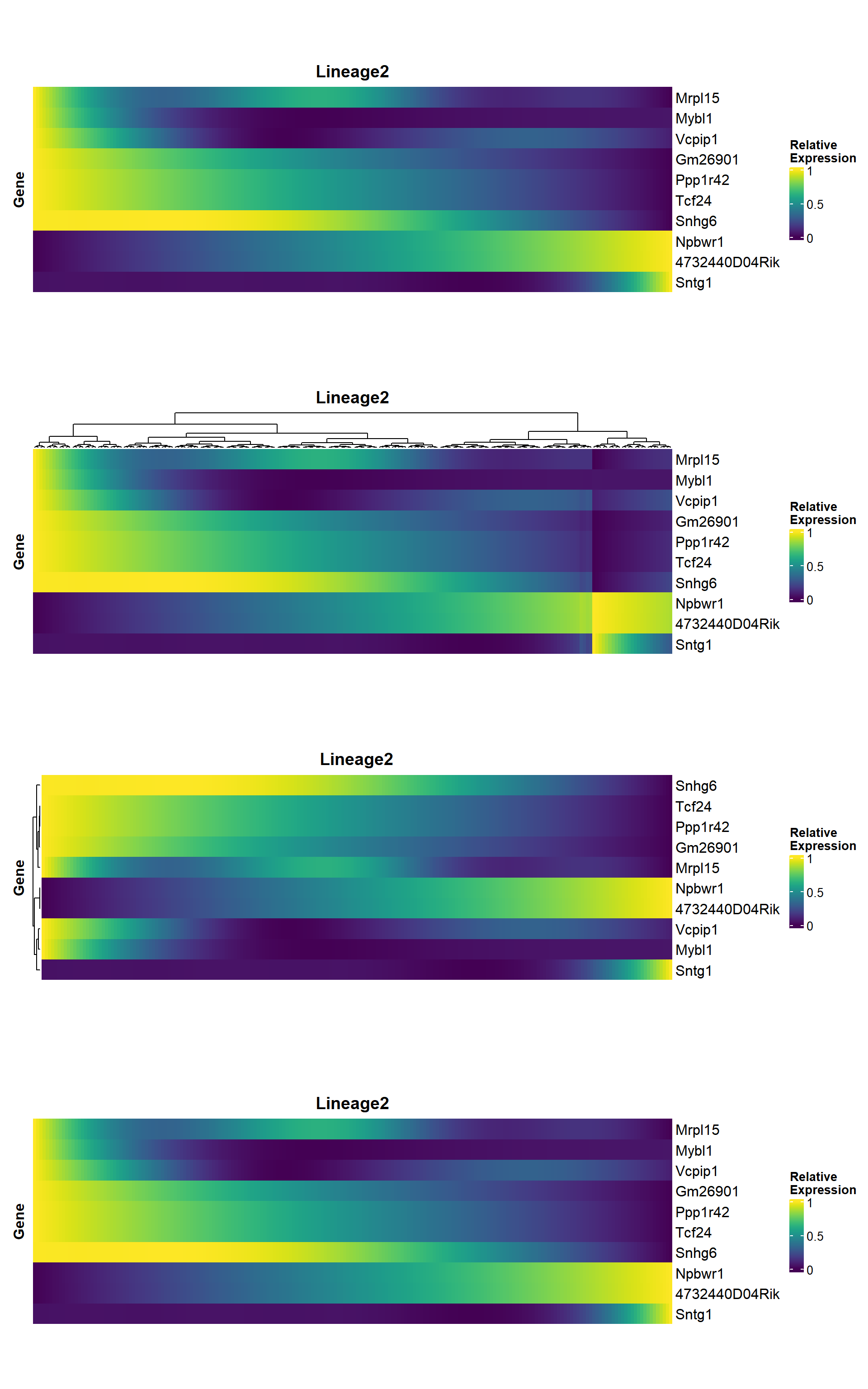

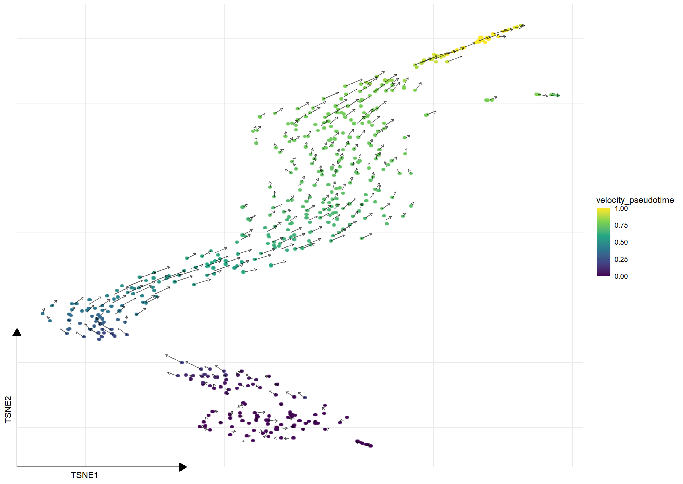
5.2 RNA velocity

RNA metabolic process:

RNA is synthesized at a rate of alpha
RNA is spliced to remove introns and form mature mRNA at rate of beta
Mature mRNA is degraded after functioning at rate of gamma

The disruption of the equilibrium between unspliced and spliced RNA indicates whether a gene is in an induced or repressed state.

With RNA-seq, especially the Poly-A enrichment method, the propotion of unspliced RNA obtained is relatively small. Currently, there are also some techinques capable of enriching nascent RNA in single cells, such as scSLAM-seq and scNT-seq.

Although some researchers are skeptical about RNA velocity, it has received significant attention because it can automatically detect the direction of trajectories.

scVelo supports a full dynamical model and various of utility functions (Bergen et al. 2020). It only supports Python and can be run in R using velociraptor.

5.2.1 Example data

This example is adopted from https://www.bioconductor.org/packages/devel/bioc/vignettes/velociraptor/inst/doc/velociraptor.html.

library(scRNAseq)
sce <- HermannSpermatogenesisData()

## Found more than one class "package_version" in cache; using the first, from namespace 'SeuratObject'

## Also defined by 'alabaster.base'

sce

## class: SingleCellExperiment 
## dim: 54448 2325 
## metadata(0):
## assays(2): spliced unspliced
## rownames(54448): ENSMUSG00000102693.1
##   ENSMUSG00000064842.1 ... ENSMUSG00000064369.1
##   ENSMUSG00000064372.1
## rowData names(0):
## colnames(2325): CCCATACTCCGAAGAG AATCCAGTCATCTGCC ...
##   ATCCACCCACCACCAG ATTGGTGGTTACCGAT
## colData names(1): celltype

## Found more than one class "package_version" in cache; using the first, from namespace 'SeuratObject'
## Also defined by 'alabaster.base'

## reducedDimNames(0):
## mainExpName: NULL

## Found more than one class "package_version" in cache; using the first, from namespace 'SeuratObject'
## Also defined by 'alabaster.base'

## altExpNames(0):

# first 500 cells for demonstration
sce <- sce[, 1:500]

## Found more than one class "package_version" in cache; using the first, from namespace 'SeuratObject'
## Also defined by 'alabaster.base'

library(scuttle)
sce <- logNormCounts(sce, assay.type=1)

## Found more than one class "package_version" in cache; using the first, from namespace 'SeuratObject'

## Also defined by 'alabaster.base'

## Found more than one class "package_version" in cache; using the first, from namespace 'SeuratObject'

## Also defined by 'alabaster.base'

library(sclet)
sce <- FindVariableFeatures(sce, method="scran")
hvgs <- VariableFeatures(sce, method="scran")

5.2.2 Run velocity analysis

library(velociraptor)

## Registered S3 method overwritten by 'zellkonverter':
##   method                                             from      
##   py_to_r.pandas.core.arrays.categorical.Categorical reticulate

velo.out <- scvelo(
  sce, subset.row=hvgs, assay.X="spliced",
  scvelo.params=list(neighbors=list(n_neighbors=30L))
)

## Found more than one class "package_version" in cache; using the first, from namespace 'SeuratObject'

## Also defined by 'alabaster.base'

## Installing pyenv ...
## Done! pyenv has been installed to '/home/runner/.local/share/r-reticulate/pyenv/bin/pyenv'.
## Using Python: /home/runner/.pyenv/versions/3.12.10/bin/python3.12
## Creating virtual environment '/home/runner/.cache/R/basilisk/1.22.0/velociraptor/1.20.0/env' ...

## + /home/runner/.pyenv/versions/3.12.10/bin/python3.12 -m venv /home/runner/.cache/R/basilisk/1.22.0/velociraptor/1.20.0/env

## Done!
## Installing packages: pip, wheel, setuptools

## + /home/runner/.cache/R/basilisk/1.22.0/velociraptor/1.20.0/env/bin/python -m pip install --upgrade pip wheel setuptools

## Installing packages: 'scvelo==0.3.3'

## + /home/runner/.cache/R/basilisk/1.22.0/velociraptor/1.20.0/env/bin/python -m pip install --upgrade --no-user 'scvelo==0.3.3'

## Virtual environment '/home/runner/.cache/R/basilisk/1.22.0/velociraptor/1.20.0/env' successfully created.
## computing moments based on connectivities
##     finished (0:00:00) --> added 
##     'Ms' and 'Mu', moments of un/spliced abundances (adata.layers)
## computing velocities
##     finished (0:00:00) --> added 
##     'velocity', velocity vectors for each individual cell (adata.layers)
## computing velocity graph (using 1/4 cores)
## WARNING: Unable to create progress bar. Consider installing `tqdm` as `pip install tqdm` and `ipywidgets` as `pip install ipywidgets`,
## or disable the progress bar using `show_progress_bar=False`.
##     finished (0:00:00) --> added 
##     'velocity_graph', sparse matrix with cosine correlations (adata.uns)
## computing terminal states
##     identified 1 region of root cells and 1 region of end points .
##     finished (0:00:00) --> added
##     'root_cells', root cells of Markov diffusion process (adata.obs)
##     'end_points', end points of Markov diffusion process (adata.obs)
## --> added 'velocity_length' (adata.obs)
## --> added 'velocity_confidence' (adata.obs)
## --> added 'velocity_confidence_transition' (adata.obs)

## For native R and reading and writing of H5AD files, an R
## <AnnData> object, and conversion to <SingleCellExperiment>
## or <Seurat> objects, check out the anndataR package:
## ℹ Install it from Bioconductor with
##   `BiocManager::install("anndataR")`
## ℹ See more at <https://bioconductor.org/packages/anndataR/>
## This message is displayed once per session.

velo.out

## class: SingleCellExperiment 
## dim: 2000 500 
## metadata(4): neighbors velocity_params velocity_graph
##   velocity_graph_neg
## assays(6): X spliced ... Mu velocity
## rownames(2000): ENSMUSG00000117819.1
##   ENSMUSG00000081984.3 ... ENSMUSG00000022965.8
##   ENSMUSG00000094660.2
## rowData names(4): velocity_gamma velocity_qreg_ratio
##   velocity_r2 velocity_genes
## colnames(500): CCCATACTCCGAAGAG AATCCAGTCATCTGCC ...
##   CACCTTGTCGTAGGAG TTCCCAGAGACTAAGT
## colData names(7): velocity_self_transition root_cells
##   ... velocity_confidence
##   velocity_confidence_transition

## Found more than one class "package_version" in cache; using the first, from namespace 'SeuratObject'
## Also defined by 'alabaster.base'

## reducedDimNames(1): X_pca
## mainExpName: NULL

## Found more than one class "package_version" in cache; using the first, from namespace 'SeuratObject'
## Also defined by 'alabaster.base'

## altExpNames(0):

5.2.3 Visualize velocity-based trajectory

library(scater)
library(sclet)
conflicted::conflicts_prefer(sclet::runPCA)

## [conflicted] Will prefer sclet::runPCA over any other
## package.

set.seed(100)
sce <- runPCA(sce, subset_row=hvgs)

## Found more than one class "package_version" in cache; using the first, from namespace 'SeuratObject'
## Also defined by 'alabaster.base'

sce <- runTSNE(sce, dimred="PCA", perplexity = 30)

## Found more than one class "package_version" in cache; using the first, from namespace 'SeuratObject'
## Also defined by 'alabaster.base'
## Found more than one class "package_version" in cache; using the first, from namespace 'SeuratObject'
## Also defined by 'alabaster.base'

sce$velocity_pseudotime <- velo.out$velocity_pseudotime

embedded <- embedVelocity(reducedDim(sce, "TSNE"), velo.out)

## Found more than one class "package_version" in cache; using the first, from namespace 'SeuratObject'
## Also defined by 'alabaster.base'
## Found more than one class "package_version" in cache; using the first, from namespace 'SeuratObject'
## Also defined by 'alabaster.base'
## Found more than one class "package_version" in cache; using the first, from namespace 'SeuratObject'
## Also defined by 'alabaster.base'
## Found more than one class "package_version" in cache; using the first, from namespace 'SeuratObject'
## Also defined by 'alabaster.base'
## ℹ Using the 'X' assay as the X matrix
## Found more than one class "package_version" in cache; using the first, from namespace 'SeuratObject'
## Also defined by 'alabaster.base'
## Found more than one class "package_version" in cache; using the first, from namespace 'SeuratObject'
## Also defined by 'alabaster.base'
## Found more than one class "package_version" in cache; using the first, from namespace 'SeuratObject'
## Also defined by 'alabaster.base'
## Found more than one class "package_version" in cache; using the first, from namespace 'SeuratObject'
## Also defined by 'alabaster.base'
## Found more than one class "package_version" in cache; using the first, from namespace 'SeuratObject'
## Also defined by 'alabaster.base'

## computing velocity embedding
##     finished (0:00:00) --> added
##     'velocity_target', embedded velocity vectors (adata.obsm)

grid.df <- gridVectors(sce, embedded, use.dimred = "TSNE")

## Found more than one class "package_version" in cache; using the first, from namespace 'SeuratObject'
## Also defined by 'alabaster.base'

require(ggsc)
sc_dim(sce, reduction='TSNE', mapping=aes(color=velocity_pseudotime)) + 
    scale_color_viridis_c() +
    geom_segment(data=grid.df, 
        mapping=aes(x=start.1, y=start.2, 
            xend=end.1, yend=end.2, colour=NULL), 
        arrow=arrow(length=unit(0.05, "inches")), alpha=.6)

## Found more than one class "package_version" in cache; using the first, from namespace 'SeuratObject'
## Also defined by 'alabaster.base'
## Found more than one class "package_version" in cache; using the first, from namespace 'SeuratObject'
## Also defined by 'alabaster.base'

References

Bergen, Volker, Marius Lange, Stefan Peidli, F. Alexander Wolf, and Fabian J. Theis. 2020. “Generalizing RNA Velocity to Transient Cell States Through Dynamical Modeling.” Nature Biotechnology 38 (12): 1408–14. https://doi.org/10.1038/s41587-020-0591-3.