10 SVP
Robust analysis of ‘gene set’ activity in spatial or single-cell data.
library(SpatialExperiment)
library(SingleCellExperiment)
library(scuttle)
library(SVP)
library(ggplot2)
library(ggsc)
10.1 runSGSA
Calculate the activity of gene sets in spatial or single-cell data with restart walk with restart and hyper test weighted. sceSubPbmc is a small SingleCellExperiment data set from pbmck3 which contains 1304 genes and 800 cells (extract randomly).
## Found more than one class "package_version" in cache; using the first, from namespace 'SeuratObject'## Also defined by 'alabaster.base'## Found more than one class "package_version" in cache; using the first, from namespace 'SeuratObject'## Also defined by 'alabaster.base'# the using runMCA to perform MCA (Multiple Correspondence Analysis)
# this is refer to the CelliD, but we using the Eigen to speed up.
# You can view the help information of runMCA using ?runMCA.
sceSubPbmc <- runMCA(sceSubPbmc, assay.type = 'logcounts')## Computing Fuzzy Matrix## Computing SVD## Computing Coordinates## Found more than one class "package_version" in cache; using the first, from namespace 'SeuratObject'## Also defined by 'alabaster.base'CellCycle.Hs is the S and G2M gene list are from the Seurat which refer to this article (doi:10.1126/science.aad050), the G1 gene list is from the G1_PHASE of Human Gene Set in MSigDB, but remove the duplicated records with S and G2M gene list.
# Next, we can calculate the activity score of gene sets provided.
# Here, we use the Cell Cycle gene set from the Seurat
# You can use other gene set, such as KEGG pathway, GO, Hallmark of MSigDB
# or TFs gene sets etc.
data(CellCycle.Hs)
sceSubPbmc <- runSGSA(sceSubPbmc, gset.idx.list = CellCycle.Hs, gsvaExp.name = 'CellCycle')
## Found more than one class "package_version" in cache; using the first, from namespace 'SeuratObject'## Also defined by 'alabaster.base'## Found more than one class "package_version" in cache; using the first, from namespace 'SeuratObject'## Also defined by 'alabaster.base'## Building the nearest neighbor graph with the distance
## between features and cells ...## elapsed time is 0.213000 seconds## Building the seed matrix using the gene set and the nearest
## neighbor graph for random walk with restart ...## elapsed time is 0.007000 seconds## Calculating the affinity score using random walk with
## restart ...## elapsed time is 0.023000 seconds## Tidying the result of random walk with restart ...## elapsed time is 0.006000 seconds## ORA analysis ...## elapsed time is 0.006000 seconds## Found more than one class "package_version" in cache; using the first, from namespace 'SeuratObject'
## Also defined by 'alabaster.base'
## Found more than one class "package_version" in cache; using the first, from namespace 'SeuratObject'
## Also defined by 'alabaster.base'
## Found more than one class "package_version" in cache; using the first, from namespace 'SeuratObject'
## Also defined by 'alabaster.base'
## Found more than one class "package_version" in cache; using the first, from namespace 'SeuratObject'
## Also defined by 'alabaster.base'
## Found more than one class "package_version" in cache; using the first, from namespace 'SeuratObject'
## Also defined by 'alabaster.base'
## class: SVPExperiment
## dim: 1304 800
## metadata(0):
## assays(2): counts logcounts
## rownames(1304): LYZ GNG7 ... TAF1 TBRG4
## rowData names(0):
## colnames(800): ACGAACTGGCTATG GGGCCAACCTTGGA ...
## TTCAAGCTAAGAAC TTACACACGTGTTG
## colData names(2): seurat_annotations sizeFactor## Found more than one class "package_version" in cache; using the first, from namespace 'SeuratObject'
## Also defined by 'alabaster.base'## reducedDimNames(1): MCA
## mainExpName: RNA## Found more than one class "package_version" in cache; using the first, from namespace 'SeuratObject'
## Also defined by 'alabaster.base'## altExpNames(0):
## spatialCoords names(0) :
## imgData names(0):
## gsvaExps names(1) : CellCycle## Found more than one class "package_version" in cache; using the first, from namespace 'SeuratObject'## Also defined by 'alabaster.base'## class: SingleCellExperiment
## dim: 3 800
## metadata(0):
## assays(1): affi.score
## rownames(3): S G2M G1
## rowData names(4): exp.gene.num gset.gene.num
## gene.occurrence.rate geneSets
## colnames(800): ACGAACTGGCTATG GGGCCAACCTTGGA ...
## TTCAAGCTAAGAAC TTACACACGTGTTG
## colData names(2): seurat_annotations sizeFactor## Found more than one class "package_version" in cache; using the first, from namespace 'SeuratObject'
## Also defined by 'alabaster.base'## reducedDimNames(0):
## mainExpName: NULL## Found more than one class "package_version" in cache; using the first, from namespace 'SeuratObject'
## Also defined by 'alabaster.base'## altExpNames(0):## Found more than one class "package_version" in cache; using the first, from namespace 'SeuratObject'
## Also defined by 'alabaster.base'## 6 x 3 sparse Matrix of class "dgCMatrix"
## S G2M G1
## ACGAACTGGCTATG . . 0.0001332757
## GGGCCAACCTTGGA . . .
## ACGAGGGACAGGAG . . .
## CAGGTTGAGGATCT . . .
## CATACTTGGGTTAC . . .
## AAGCCATGAACTGC . . .# Then you can use the ggsc or other package to visulize
# and you can try to use the findMarkers of scran or other packages to identify
# the different gene sets.
sceSubPbmc <- sceSubPbmc |>
scater::runPCA(assay.type = 'logcounts', ntop = 600) |>
scater::runUMAP(dimred = 'PCA')## Found more than one class "package_version" in cache; using the first, from namespace 'SeuratObject'## Also defined by 'alabaster.base'## Found more than one class "package_version" in cache; using the first, from namespace 'SeuratObject'## Also defined by 'alabaster.base'## Found more than one class "package_version" in cache; using the first, from namespace 'SeuratObject'## Also defined by 'alabaster.base'# withReducedDim = TRUE, the original reducetion results from original gene features
# will be add the colData in the sce.cellcycle.
sce.cellcycle <- sceSubPbmc |> gsvaExp('CellCycle', withReducedDim=TRUE)## Found more than one class "package_version" in cache; using the first, from namespace 'SeuratObject'
## Also defined by 'alabaster.base'## Found more than one class "package_version" in cache; using the first, from namespace 'SeuratObject'## Also defined by 'alabaster.base'## Found more than one class "package_version" in cache; using the first, from namespace 'SeuratObject'## Also defined by 'alabaster.base'## class: SingleCellExperiment
## dim: 3 800
## metadata(0):
## assays(1): affi.score
## rownames(3): S G2M G1
## rowData names(4): exp.gene.num gset.gene.num
## gene.occurrence.rate geneSets
## colnames(800): ACGAACTGGCTATG GGGCCAACCTTGGA ...
## TTCAAGCTAAGAAC TTACACACGTGTTG
## colData names(2): seurat_annotations sizeFactor## Found more than one class "package_version" in cache; using the first, from namespace 'SeuratObject'
## Also defined by 'alabaster.base'## reducedDimNames(3): MCA PCA UMAP
## mainExpName: NULL## Found more than one class "package_version" in cache; using the first, from namespace 'SeuratObject'
## Also defined by 'alabaster.base'## altExpNames(0):sce.cellcycle |> sc_violin(
features = rownames(sce.cellcycle),
mapping = aes(x=seurat_annotations, fill = seurat_annotations)
) +
scale_x_discrete(guide=guide_axis(angle=-45))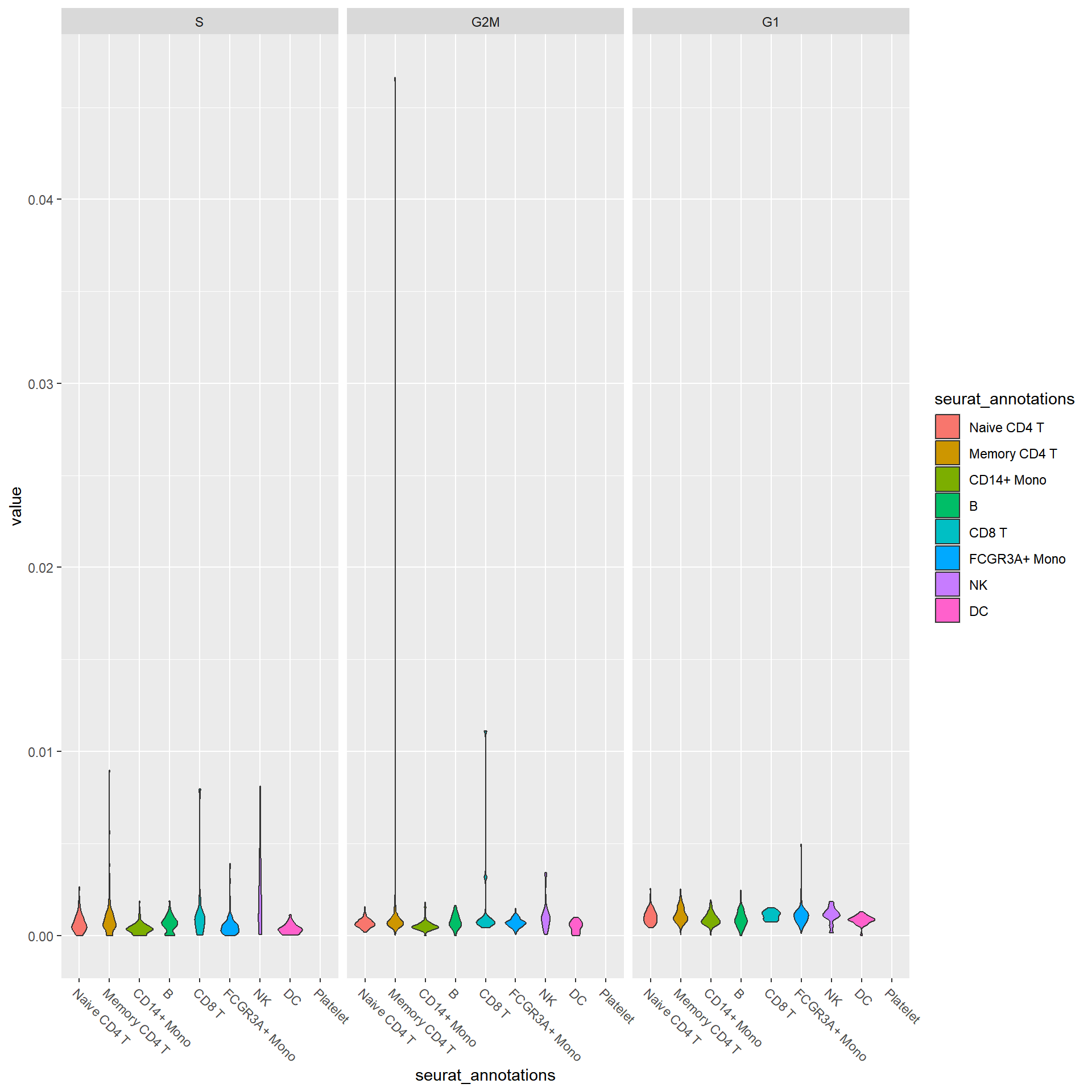
## Found more than one class "package_version" in cache; using the first, from namespace 'SeuratObject'## Also defined by 'alabaster.base'## Found more than one class "package_version" in cache; using the first, from namespace 'SeuratObject'## Also defined by 'alabaster.base'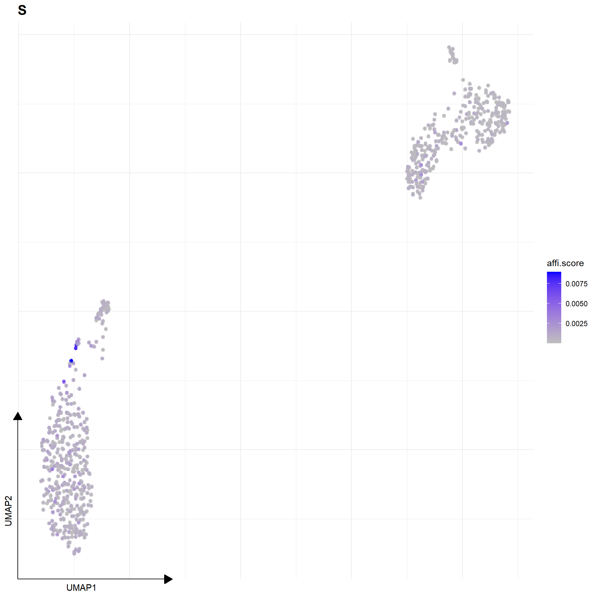
library(scran)
cellcycle.test.res <- sce.cellcycle |> findMarkers(
                group = sce.cellcycle$seurat_annotations,
                test.type = 'wilcox',
                assay.type = 'affi.score',
                add.summary = TRUE
                )
cellcycle.test.res$B
## DataFrame with 3 rows and 16 columns
## self.average other.average self.detected other.detected
## <numeric> <numeric> <numeric> <numeric>
## S 8.66873e-08 6.06313e-06 0.0222222 0.0852919
## G2M 1.54464e-06 3.07913e-05 0.2888889 0.2456323
## G1 3.85454e-07 1.75387e-05 0.0666667 0.2132489
## Top p.value FDR summary.AUC
## <integer> <numeric> <numeric> <numeric>
## S 1 0.00269317 0.00807951 0.325253
## G2M 1 0.04878874 0.04878874 0.589790
## G1 1 0.00558551 0.00837826 0.000000
## AUC.Naive CD4 T AUC.Memory CD4 T AUC.CD14+ Mono
## <numeric> <numeric> <numeric>
## S 0.490991 0.482074 0.500926
## G2M 0.589790 0.543111 0.539583
## G1 0.487688 0.483457 0.469907
## AUC.CD8 T AUC.FCGR3A+ Mono AUC.NK AUC.DC
## <numeric> <numeric> <numeric> <numeric>
## S 0.423529 0.499658 0.325253 0.511111
## G2M 0.560784 0.472821 0.301010 0.607885
## G1 0.533333 0.427009 0.486869 0.483154
## AUC.Platelet
## <numeric>
## S 0.511111
## G2M 0.644444
## G1 0.00000010.2 runLISA
hpda_spe_cell_dec is the result of runSGSA with HPDA A sample from (doi:10.1038/s41587-019-0392-8). Each item in the matrix is the marker gene set activity in the spot. The marker gene set represents the cell type. We can use svp the investigate if a cell type cluters and if two cell types appear in the same region. Usage of local indicators of spatial association (LISA) to identify the hotspot in the spatial space
data(hpda_spe_cell_dec)

# r$> assay(hpda_spe_cell_dec)[1:5,1:5]
# 5 x 5 sparse Matrix of class "dgCMatrix"
#                                             Spot1        Spot2        Spot3        Spot4        Spot5
# Acinar cells                         3.283881e-04 6.931743e-06 4.820951e-05 1.882577e-03 9.269843e-04
# Cancer clone A                       2.880388e-04 2.013973e-04 9.167013e-05 9.642225e-05 6.704812e-05
# Cancer clone B                       1.569730e-04 2.744810e-04 2.151324e-04 1.502651e-05 4.283322e-06
# Ductal APOL1 high-hypoxic            3.132481e-05 3.902286e-04 4.240874e-05 3.140970e-06 1.464118e-04
# Ductal CRISP3 high-centroacinar like 9.546611e-05 5.025320e-03 2.112512e-03 1.140155e-03 3.873088e-03

svres <- runDetectSVG(hpda_spe_cell_dec, assay.type = 'affi.score',
                      method = 'moransi', action = 'only')
## Found more than one class "package_version" in cache; using the first, from namespace 'SeuratObject'## Also defined by 'alabaster.base'## Identifying the spatially variable gene sets (pathway)
## based on moransi## elapsed time is 0.029000 seconds# r$> svres |> dplyr::arrange(rank) |> head()
# obs expect.moransi sd.moransi Z.moransi pvalue padj rank
# Cancer clone A 0.7086916 -0.00234192 0.02803920 25.35855 3.616015e-142 7.232030e-141 1
# Acinar cells 0.6958980 -0.00234192 0.02788076 25.04379 1.020141e-138 1.020141e-137 2
# Cancer clone B 0.6586104 -0.00234192 0.02803039 23.57985 3.102650e-123 2.068434e-122 3
# mDCs A 0.5824019 -0.00234192 0.02760394 21.18334 6.801396e-100 3.400698e-99 4
# Ductal CRISP3 high-centroacinar like 0.5605955 -0.00234192 0.02794187 20.14673 1.437344e-90 5.749375e-90 5
# Endothelial cells 0.5362475 -0.00234192 0.02757573 19.53128 2.976221e-85 9.920735e-85 6lisa.res12 <- hpda_spe_cell_dec |>
runLISA(
features = c(1, 2, 3),
assay.type = 'affi.score',
weight.method = "knn",
k = 10,
action = 'get',
)## Found more than one class "package_version" in cache; using the first, from namespace 'SeuratObject'## Also defined by 'alabaster.base'## List of length 3
## names(3): Acinar cells Cancer clone A Cancer clone B## Gi E.Gi Var.Gi Z.Gi
## Spot1 0.0003594390 0.00234192 1.553580e-06 -1.5905315
## Spot2 0.0009293147 0.00234192 1.551111e-06 -1.1342257
## Spot3 0.0010726076 0.00234192 1.551438e-06 -1.0190641
## Spot4 0.0009029930 0.00234192 1.563140e-06 -1.1509064
## Spot5 0.0011642594 0.00234192 1.557730e-06 -0.9435702
## Spot6 0.0008351924 0.00234192 1.551895e-06 -1.2094939
## Pr (z != E(Gi)) cluster.no.test cluster.test
## Spot1 0.1117150 Low NoSign
## Spot2 0.2566999 Low NoSign
## Spot3 0.3081725 Low NoSign
## Spot4 0.2497708 Low NoSign
## Spot5 0.3453893 Low NoSign
## Spot6 0.2264732 Low NoSign## Gi E.Gi Var.Gi Z.Gi
## Spot1 0.0004249351 0.00234192 1.394101e-06 -1.623573
## Spot2 0.0003356962 0.00234192 1.393067e-06 -1.699783
## Spot3 0.0004122264 0.00234192 1.391701e-06 -1.635745
## Spot4 0.0004537437 0.00234192 1.391761e-06 -1.600517
## Spot5 0.0004554667 0.00234192 1.391386e-06 -1.599272
## Spot6 0.0006432991 0.00234192 1.393284e-06 -1.439053
## Pr (z != E(Gi)) cluster.no.test cluster.test
## Spot1 0.10446707 Low NoSign
## Spot2 0.08917177 Low NoSign
## Spot3 0.10189306 Low NoSign
## Spot4 0.10948398 Low NoSign
## Spot5 0.10976015 Low NoSign
## Spot6 0.15013551 Low NoSigncolData(hpda_spe_cell_dec)$`cluster.test.Cancer.A` <- lisa.res12[["Cancer clone A"]] |>
dplyr::pull(cluster.test)
colData(hpda_spe_cell_dec)$`cluster.test.Acinar` <- lisa.res12[["Acinar cells"]] |>
dplyr::pull(cluster.test)
colData(hpda_spe_cell_dec)$`cluster.test.Cancer.B` <- lisa.res12[["Cancer clone B"]] |>
dplyr::pull(cluster.test)p1 <- sc_spatial(hpda_spe_cell_dec,
features = rownames(hpda_spe_cell_dec),
mapping = aes(x=x, y=y, color=cluster.test.Cancer.A),
plot.pie = T,
pie.radius.scale = .8,
bg_circle_radius = 1.1,
color=NA,
linewidth=2
) + scale_color_manual(values=c("black", "white"))
p1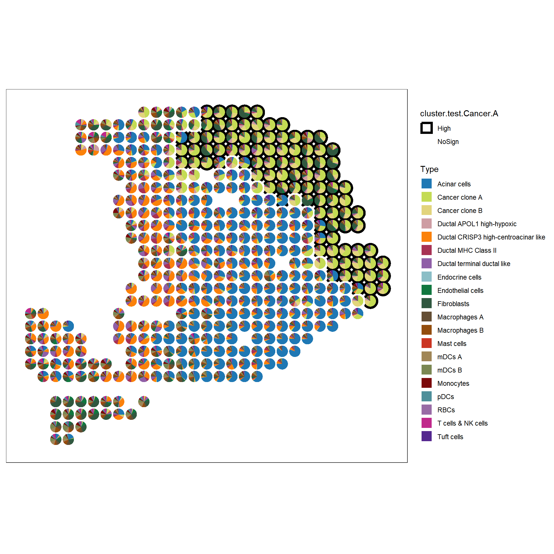
f1 <- sc_spatial(hpda_spe_cell_dec, features="Cancer clone A",
            mapping=aes(x = x, y = y),
            pointsize=10) +
        geom_scattermore2(mapping = aes(bg_color=cluster.test.Cancer.A,
                          subset=cluster.test.Cancer.A=="High"),
                          bg_line_width = .16,
                          gap_line_width = .14,
                          pointsize = 7) +
        scale_bg_color_manual(values=c('black'))
f1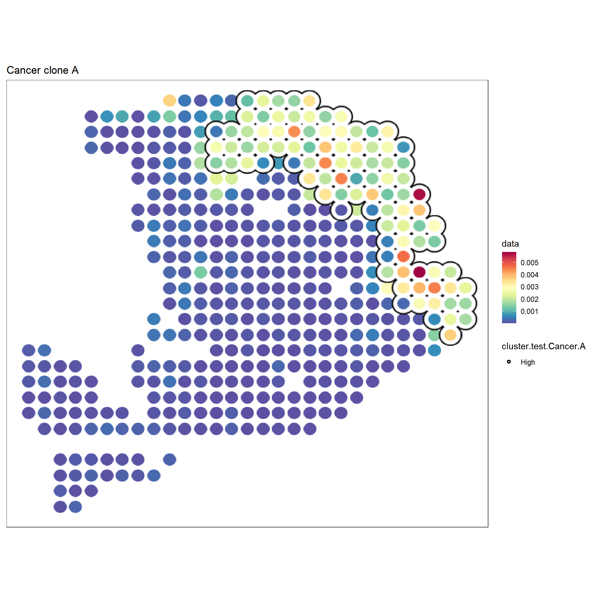
f2 <- sc_spatial(hpda_spe_cell_dec, features="Acinar cells",
            mapping=aes(x=x,y=y),
            pointsize=10) +
        geom_scattermore2(mapping = aes(bg_color=cluster.test.Acinar, subset=cluster.test.Acinar=="High"),
                          bg_line_width = .16,
                          gap_line_width = .14,
                          pointsize = 7) +
        scale_bg_color_manual(values=c('black'))
f2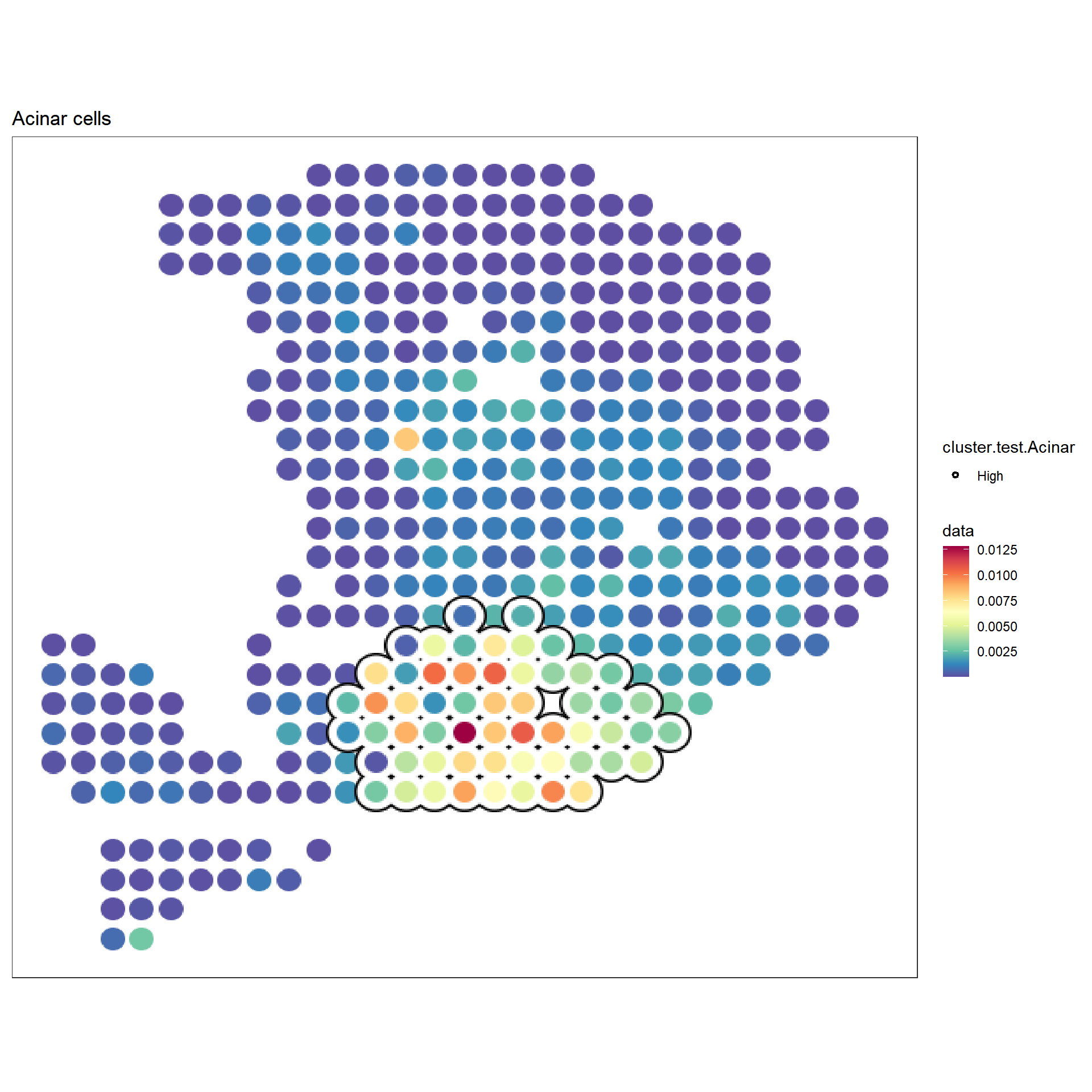
f3 <- sc_spatial(hpda_spe_cell_dec, features="Cancer clone B",
            mapping=aes(x=x,y=y),
            pointsize=10) +
        geom_scattermore2(mapping = aes(bg_color=cluster.test.Cancer.B, subset=cluster.test.Cancer.B=="High"),
                          bg_line_width = .18,
                          gap_line_width = .14,
                          pointsize = 8) +
        scale_bg_color_manual(values=c('black'))
f3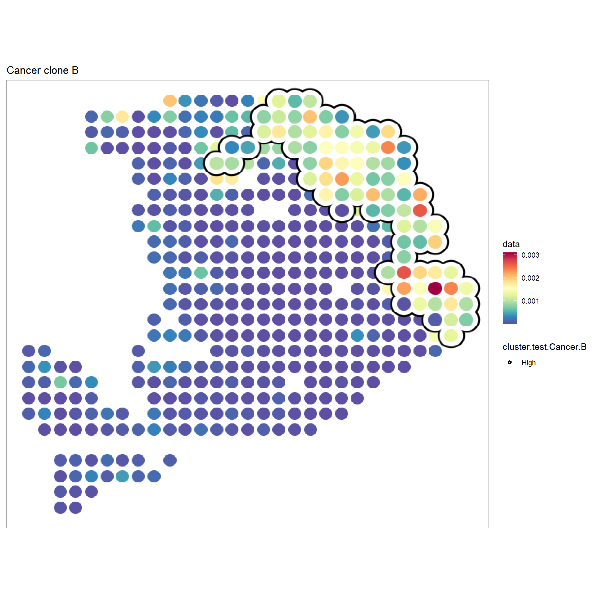
10.3 runLOCALBV
explore the local bivariate relationship in the spatial space.
res1 <- hpda_spe_cell_dec |> runLOCALBV(
          features1 = 'Cancer clone A',
          features2 = 'Cancer clone B',
          assay.type='affi.score'
        )
res1
res1[['Cancer clone A_VS_Cancer clone B']] |> head()


#        LocalLee           Gi       E.Gi       Var.Gi       Z.Gi Pr (z > E(Gi)) cluster.no.test cluster.test
# Spot1 0.2656572 0.0007993283 0.00234192 1.685012e-06 -1.1883644      0.8826551             Low       NoSign
# Spot2 0.1928726 0.0006520670 0.00234192 3.060135e-06 -0.9660035      0.8329788             Low       NoSign
# Spot3 0.2098906 0.0007134499 0.00234192 2.544445e-06 -1.0209003      0.8463492             Low       NoSign
# Spot4 0.2609793 0.0007131499 0.00234192 2.545557e-06 -1.0208654      0.8463409             Low       NoSign
# Spot5 0.1769749 0.0007300670 0.00234192 3.059710e-06 -0.9214789      0.8215998             Low       NoSign
# Spot6 0.1736672 0.0004656579 0.00234192 2.175086e-06 -1.2721999      0.8983489             Low       NoSign