A Frequently asked questions
A.1 How to prepare your own geneList
GSEA analysis requires a ranked gene list, which contains three features:
- numeric vector: fold change or other type of numerical variable
- named vector: every number has a name, the corresponding gene ID
- sorted vector: number should be sorted in decreasing order
If you import your data from a csv file, the file should contains two columns, one for gene ID (no duplicated ID allowed) and another one for fold change. You can prepare your own geneList via the following command:
d = read.csv(your_csv_file)
## assume 1st column is ID
## 2nd column is FC

## feature 1: numeric vector
geneList = d[,2]

## feature 2: named vector
names(geneList) = as.character(d[,1])

## feature 3: decreasing orde
geneList = sort(geneList, decreasing = TRUE)A.3 Showing specific pathways
By default, all the visualization methods provided by enrichplot display most significant pathways. If users are interested to show some specific pathways (e.g. excluding some unimportant pathways among the top categories), users can pass a vector of selected pathways to the showCategory parameter in dotplot(), barplot(), treeplot(), cnetplot() and emapplot() etc.
library(DOSE)
library(enrichplot)
data(geneList)
de <- names(geneList)[1:100]

x <- enrichDO(de)

## show top 10 most significant pathways and want to exclude the second one
## dotplot(x, showCategory = x$Description[1:10][-2])

set.seed(2020-10-27)
selected_pathways <- sample(x$Description, 10)
selected_pathways
## [1] "in situ carcinoma"
## [2] "hypersensitivity reaction type IV disease"
## [3] "lymph node disease"
## [4] "esophageal carcinoma"
## [5] "atopic dermatitis"
## [6] "pulmonary sarcoidosis"
## [7] "esophageal cancer"
## [8] "Human immunodeficiency virus infectious disease"
## [9] "ovarian cancer"
## [10] "breast carcinoma"
p1 <- dotplot(x, showCategory = 10, font.size=14)
p2 <- dotplot(x, showCategory = selected_pathways, font.size=14)


cowplot::plot_grid(p1, p2, labels=LETTERS[1:2])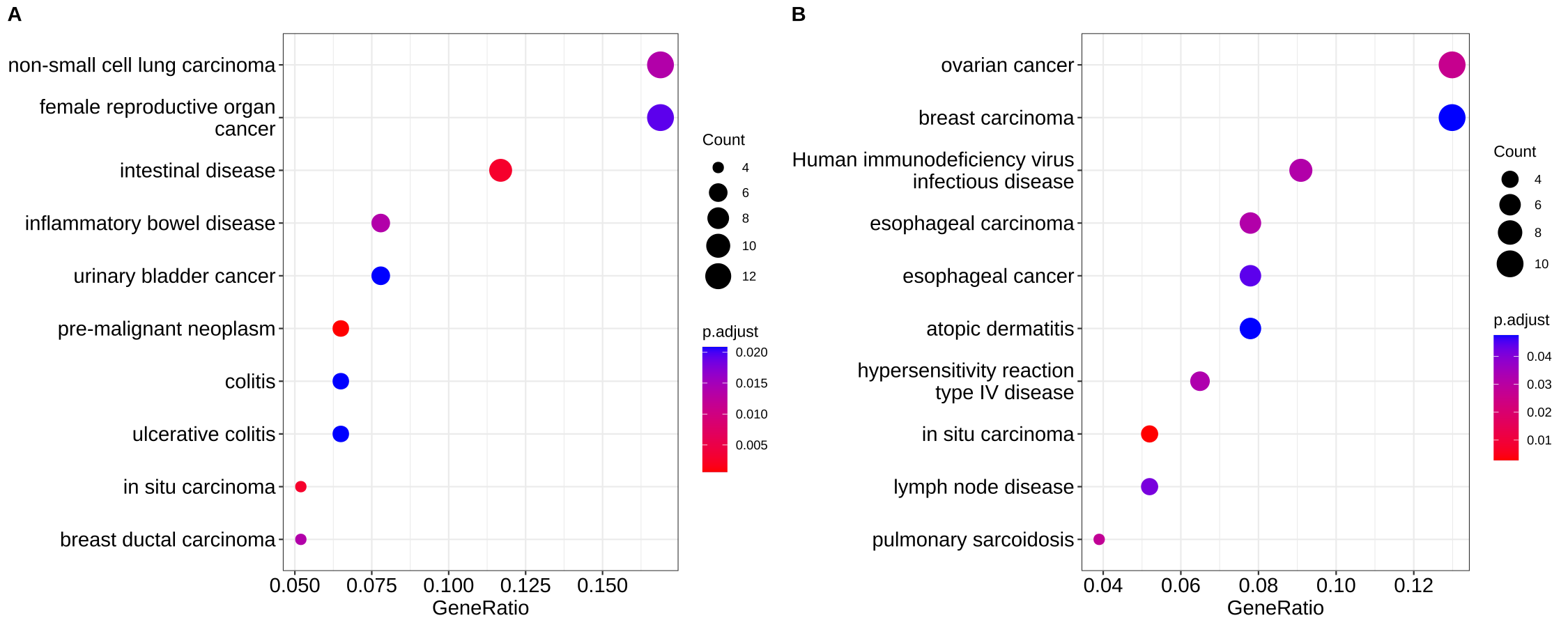
Figure A.1: Showing specific pathways. Top ten most significant pathways (A), selected ten pathways (B).
Note: Another solution is using the filter verb to extract a subset of the result as described in Chapter 16.
A.4 How to extract genes of a specific term/pathway
id <- x$ID[1:3]
id
## [1] "DOID:0060071" "DOID:5295" "DOID:8719"
x[[id[1]]]## [1] "6280" "6278" "10232" "332" "4321"
geneInCategory(x)[id]## $`DOID:0060071`
## [1] "6280" "6278" "10232" "332" "4321"
##
## $`DOID:5295`
## [1] "4312" "6279" "3627" "10563" "4283" "890" "366" "4902" "3620"
##
## $`DOID:8719`
## [1] "6280" "6278" "10232" "332"A.5 Wrap long axis labels
Most of the functions in enrichplot can automatically split long labels across multiple lines. Users can passed a line width to the label_format parameter (default is 30). It also supports user defined function to format label strings.
library(ReactomePA)
y <- enrichPathway(de)

p1 <- dotplot(y, label_format = 20)
p2 <- dotplot(y, label_format = function(x) stringr::str_wrap(x, width=20))
cowplot::plot_grid(p1, p2, ncol=2, labels=c("A", "B")) 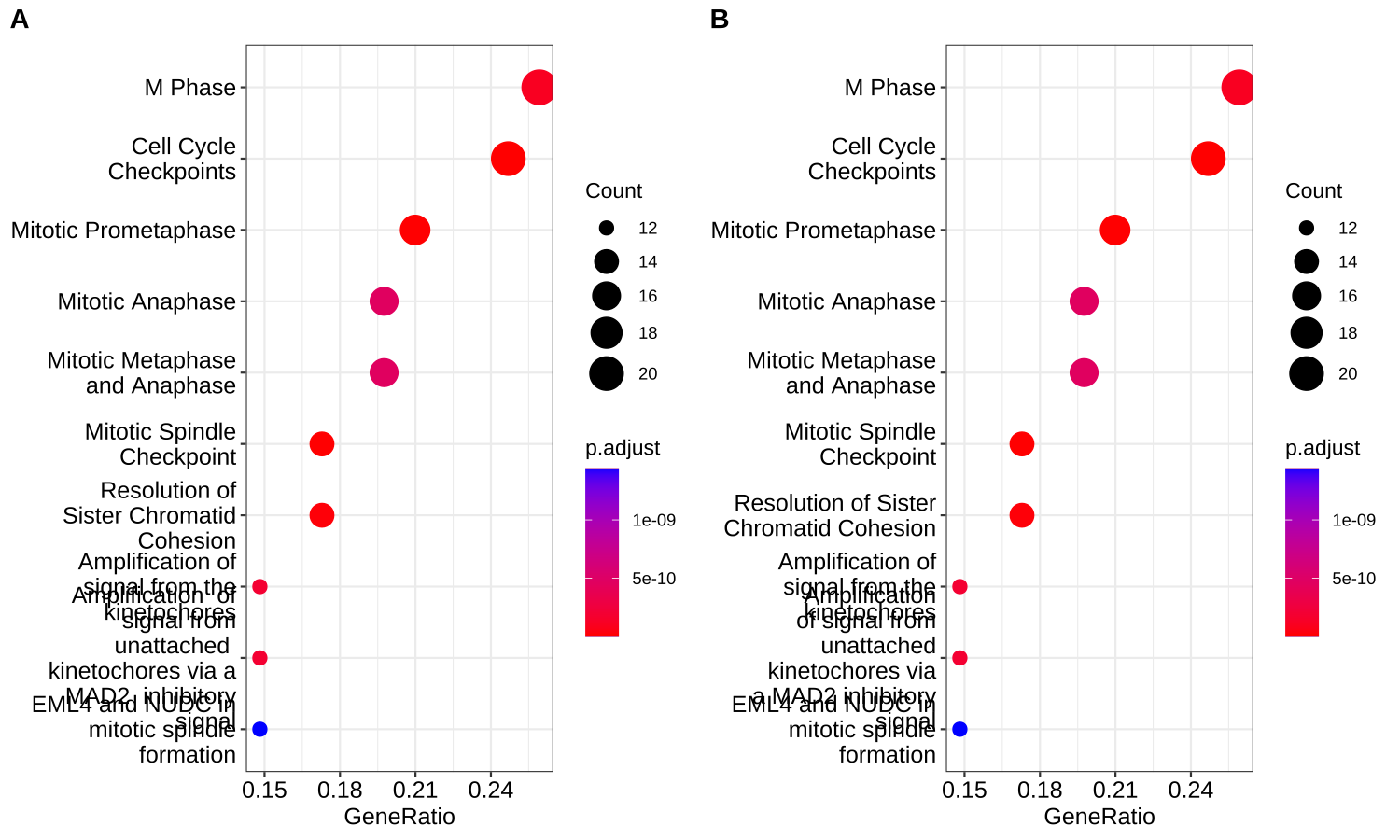
Figure A.2: Wrap long axis labels. Passing a numeric value to specify string width (A), a user specifiable labeller function (B).
The label_format option works with barplot(), dotplot(), heatplot(), treeplot and ridgeplot().