The previous two chapters drew trees from phylo and treedata objects. Those are not the only tree classes in R: other packages define their own, each shaped around the data its discipline cares about. This chapter shows that ggtree() works with them directly, so a reader whose tree comes from clustering, ecology, microbiome sequencing, or a general graph package does not need to abandon it or convert it by hand. The chapter closes with tree structures that have no dedicated class at all.
7.2 ggtree for Phylogenetic Tree Objects
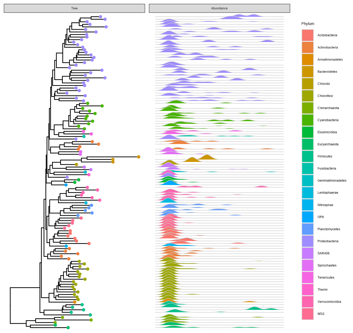
The treeio packages (Wang et al., 2020) allow parsing evolutionary inferences from several software outputs and linking external data to the tree structure. It serves as an infrastructure to bring evolutionary data to the R community. The ggtree package (Yu et al., 2017) works seamlessly with treeio to visualize tree-associated data to annotate the tree. The ggtree package is a general tool for tree visualization and annotation and it fits the ecosystem of R packages. Most of the S3/S4 tree objects defined by other R packages are also supported by ggtree, including phylo (session 5.2), multiPhylo (session 6.6), phylo4, phylo4d, phyloseq, and obkData. With ggtree, we are able to generate more complex tree graphs which is not possible or easy to do with other packages. For example, the visualization of the phyloseq object in Figure Figure 7.4 is not supported by the phyloseq package. The ggtree package also extends the possibility of linking external data to these tree objects (Yu et al., 2018).
7.2.1 The phylo4 and phylo4d objects
The phylo4 and phylo4d are defined in the phylobase package. The phylo4 object is an S4 version of phylo, while phylo4d extends phylo4 with a data frame that contains trait data. The phylobase package provides a plot() method, which is internally called the treePlot() function, to display the tree with the data. However, there are some restrictions of the plot() method, it can only plot numeric values for tree-associated data as bubbles and cannot generate figure legend. Phylobase doesn’t implement a visualization method to display categorical values. Using associated data as visual characteristics such as color, size, and shape, is also not supported. Although it is possible to color the tree using associated data, it requires users to extract the data and map them to the color vector manually followed by passing the color vector to the plot method. This is tedious and error-prone since the order of the color vector needs to be consistent with the edge list stored in the object.
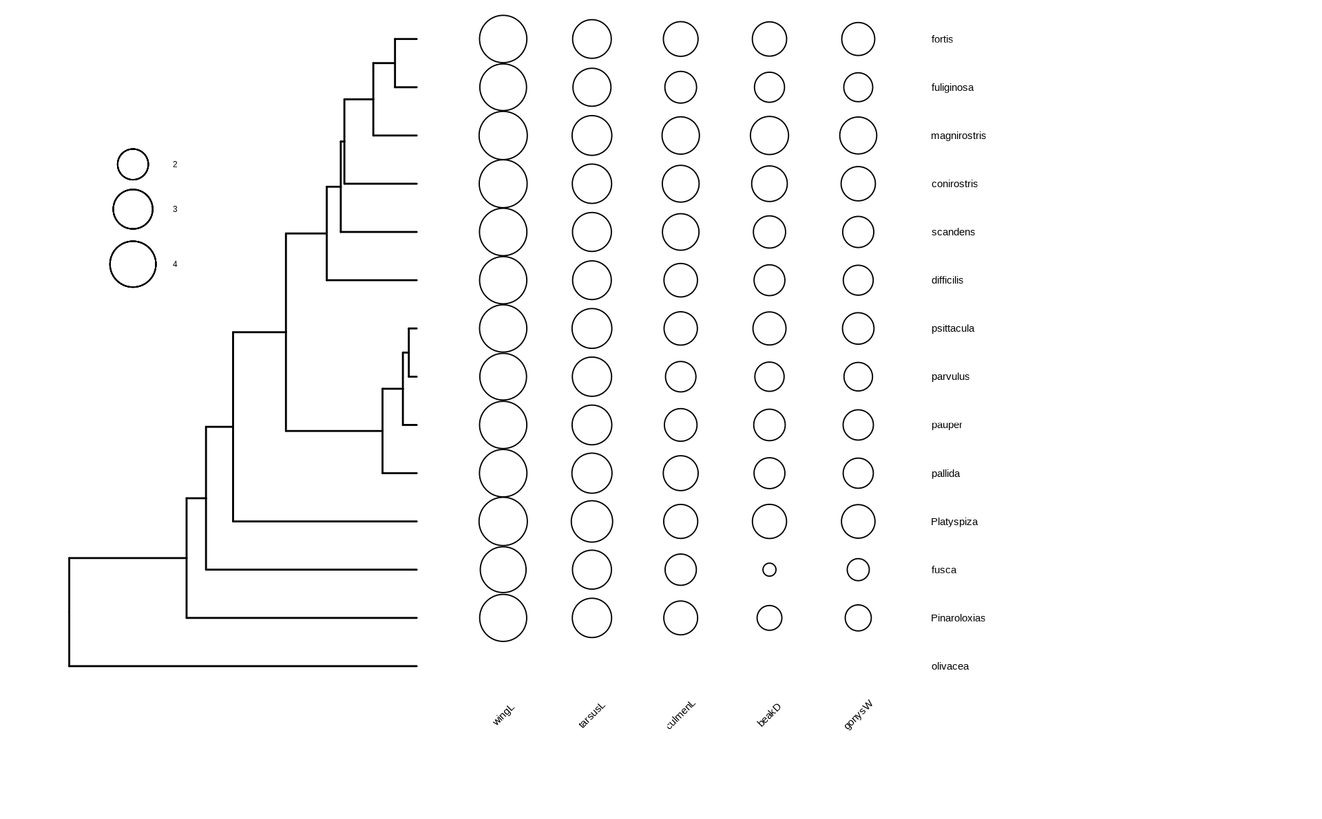
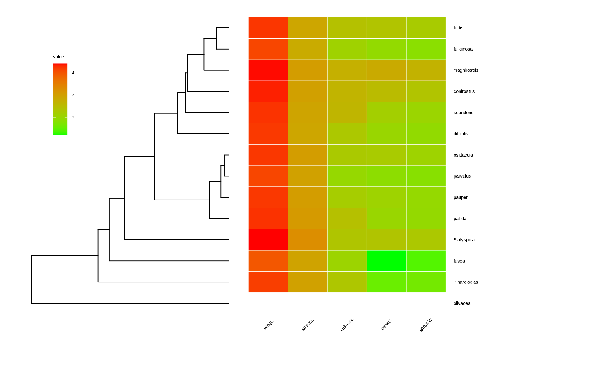
The ggtree package supports phylo4d object and all the associated data stored in the phylo4d object can be used directly to annotate the tree (Figure Figure 7.1).
library(phylobase)data(geospiza_raw)g1 <-as(geospiza_raw$tree, "phylo4")g2 <-phylo4d(g1, geospiza_raw$data, missing.data="warn")d1 <-data.frame(x =seq(1.1, 2, length.out =5),lab =names(geospiza_raw$data))p1 <-ggtree(g2) +geom_tippoint(aes(size = wingL), x = d1$x[1], shape =1) +geom_tippoint(aes(size = tarsusL), x = d1$x[2], shape =1) +geom_tippoint(aes(size = culmenL), x = d1$x[3], shape =1) +geom_tippoint(aes(size = beakD), x = d1$x[4], shape =1) +geom_tippoint(aes(size = gonysW), x = d1$x[5], shape =1) +scale_size_continuous(range =c(3,12), name="") +geom_text(aes(x = x, y =0, label = lab), data = d1, angle =45) +geom_tiplab(offset =1.3) +xlim(0, 3) +theme(legend.position =c(.1, .75)) +vexpand(.05, -1) ## users can use `as.treedata(g2)` to convert `g2` to a `treedata` object## and use `get_tree_data()` function to extract the associated data p2 <-gheatmap(ggtree(g1), data=geospiza_raw$data, colnames_angle=45) +geom_tiplab(offset=1) +hexpand(.2) +vexpand(.05, -1) +theme(legend.position =c(.1, .75))p1p2
(a) Reproduce the output of the plot() method provided in the phylobase package
(b) Visualize trait data as a heatmap, which is not supported in phylobase
Figure 7.1: Visualizing phylo4d data using ggtree.
7.2.2 The phylog object
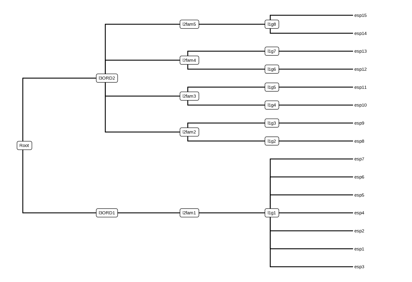
The phylog is defined in the ade4 package. The package is designed for analyzing ecological data and provides newick2phylog(), hclust2phylog(), and taxo2phylog() functions to create phylogeny from Newick string, hierarchical clustering result, or a taxonomy (see also the MicrobiotaProcess package described in Chapter 14). The phylog object is also supported by ggtree as demonstrated in Figure Figure 7.2.
Phylogenetic tree with 15 leaves and 16 nodes
$class: phylog
$call: taxo2phylog(taxo = as.taxo(taxo.eg[[1]]))
$tre: ((((esp3,esp1,esp2,esp4,e...15)l1g8)l2fam5)l3ORD2)Root;

        class   length content
$leaves numeric 15     length of the first preceeding adjacent edge
$nodes  numeric 16     length of the first preceeding adjacent edge
$parts  list    16     subsets of descendant nodes
$paths  list    31     path from root to node or leave
$droot  numeric 31     distance to root
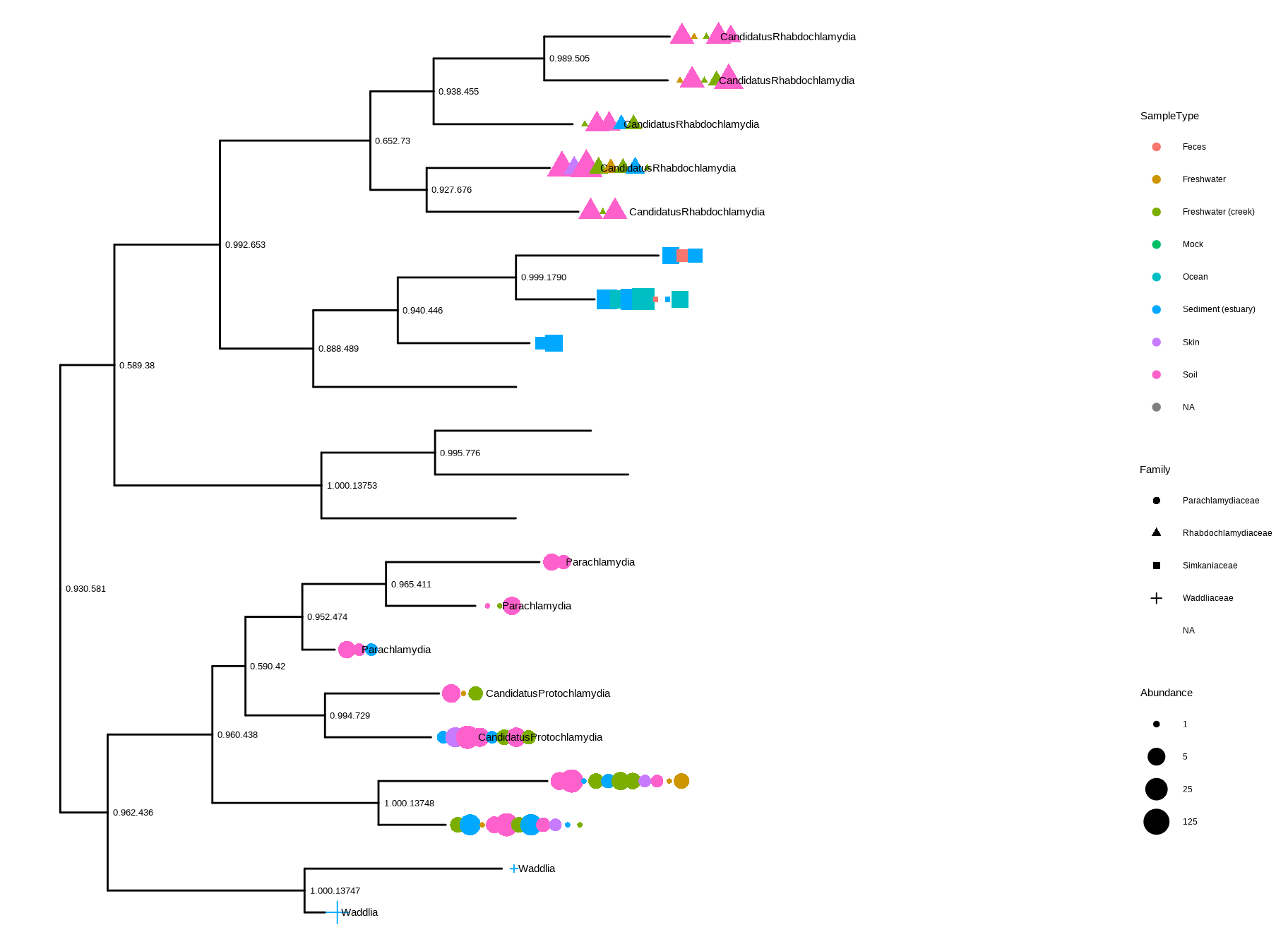
Figure 7.3: Visualizing a phyloseq tree object. This example mimics the output of the plot_tree() function provided in the r Biocpkg("phyloseq") package.
Figure Figure 7.3 reproduces the output of the phyloseq::plot_tree() function. Users of phyloseq will find ggtree useful for visualizing microbiome data and for further annotation since ggtree supports high-level annotation using the grammar of graphics and can add tree data layers that are not available in phyloseq.
Figure 7.4: Phylogenetic tree with OTU abundance densities. Tips were colored by Phylum, and the corresponding abundances across different samples were visualized as density ridgelines and sorted according to the tree structure.
This example uses microbiome data provided in the phyloseq package and density ridgeline is employed to visualize species abundance data. The geom_facet() layer automatically re-arranges the abundance data according to the tree structure, visualizes the data using the specified geom function, i.e., geom_density_ridges(), and aligns the density curves with the tree as demonstrated in Figure Figure 7.4. Note that data stored in the phyloseq object is visible to ggtree() and can be used directly in tree visualization (Phylum was used to color tips and density ridgelines in this example). The source code of this example was firstly published in the supplemental file of (Yu et al., 2018).
7.2.4 The obkData object
The okbData is defined in the OutbreakTools package to store incidence-based outbreak data, including meta data of sampling and information of infected individuals such as age and onset of symptoms. The ggtree supports the obkData object and the information can be used to annotate the tree as shown in the following example.
Hierarchical clustering is one of the most common sources of trees outside evolutionary biology: stats::hclust() and similar functions produce dendrograms that can be visualized directly with ggtree().
A dendrogram is a tree diagram to display hierarchical clustering and classification/regression trees. In R, we can calculate a hierarchical clustering using the function hclust().
hc <-hclust(dist(mtcars))hc
Call:
hclust(d = dist(mtcars))

Cluster method   : complete
Distance         : euclidean
Number of objects: 32
The hclust object describes the tree produced by the clustering process. It can be converted to dendrogram object, which stores the tree as deeply-nested lists.
den <-as.dendrogram(hc)den
'dendrogram' with 2 branches and 32 members total, at height 425.3447
Table 7.1: Supported tree-like objects in r Biocpkg("ggtree").
Object
Package
phylo
ape
multiPhylo
ape
phylo4
phylobase
phylo4d
phylobase
phyloseq
phyloseq
obkData
OutbreakTools
hclust
stats
dendrogram
stats
agnes
cluster
diana
cluster
twins
cluster
pvclust
pvclust
igraph (tree graph)
igraph
The ggtree package supports most of the hierarchical clustering objects defined in the R community, including hclust and dendrogram as well as agnes, diana, and twins that are defined in the cluster package, and the pvclust object defined in the pvclust package (Table Table 7.1). Users can use ggtree(object) to display its tree structure, and use other layers and utilities to customize the graph and of course, add annotations to the tree.
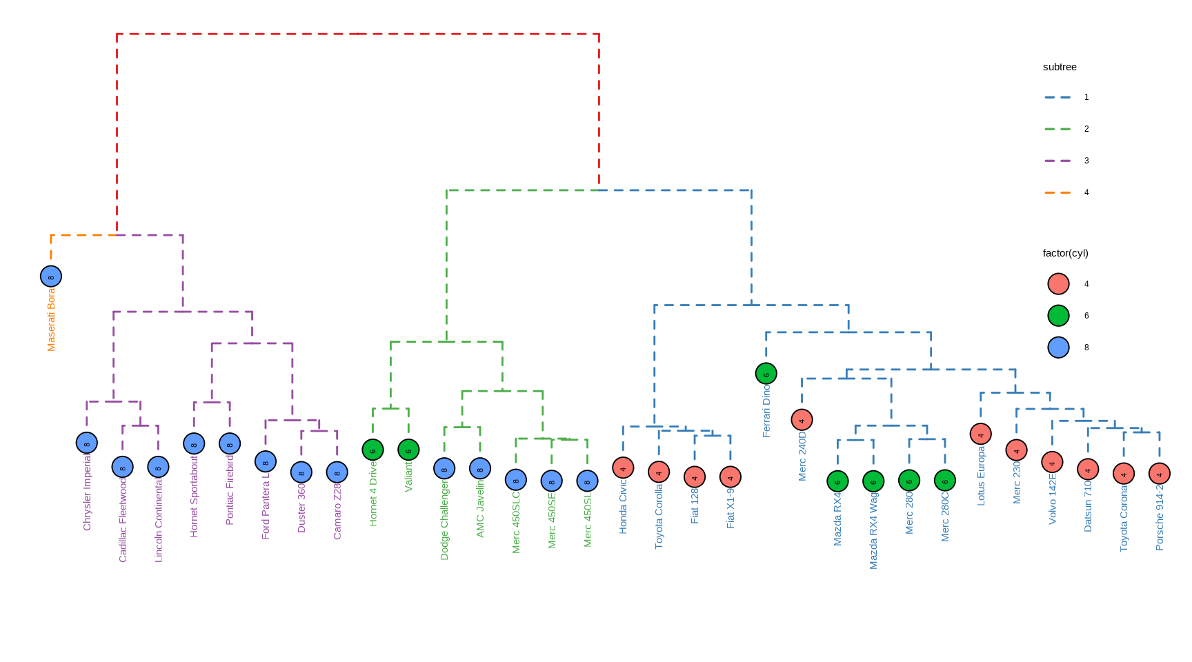
The ggtree provides layout_dendrogram() to layout the tree top-down, and theme_dendrogram() to display tree height (similar to theme_tree2() for phylogenetic tree) as demonstrated in Figure Figure 7.5 (see also the example in (Yu, 2020)).
Figure 7.5: Visualizing dendrogram. Use cutree() to split the tree into several groups and groupClade() to assign this grouping information. The tree was displayed in the classic top-down layout with branches colored by the grouping information and the tips were colored and labeled by the number of cylinders.
MRCA = tidytree::MRCA
7.4 ggtree for Tree Graph
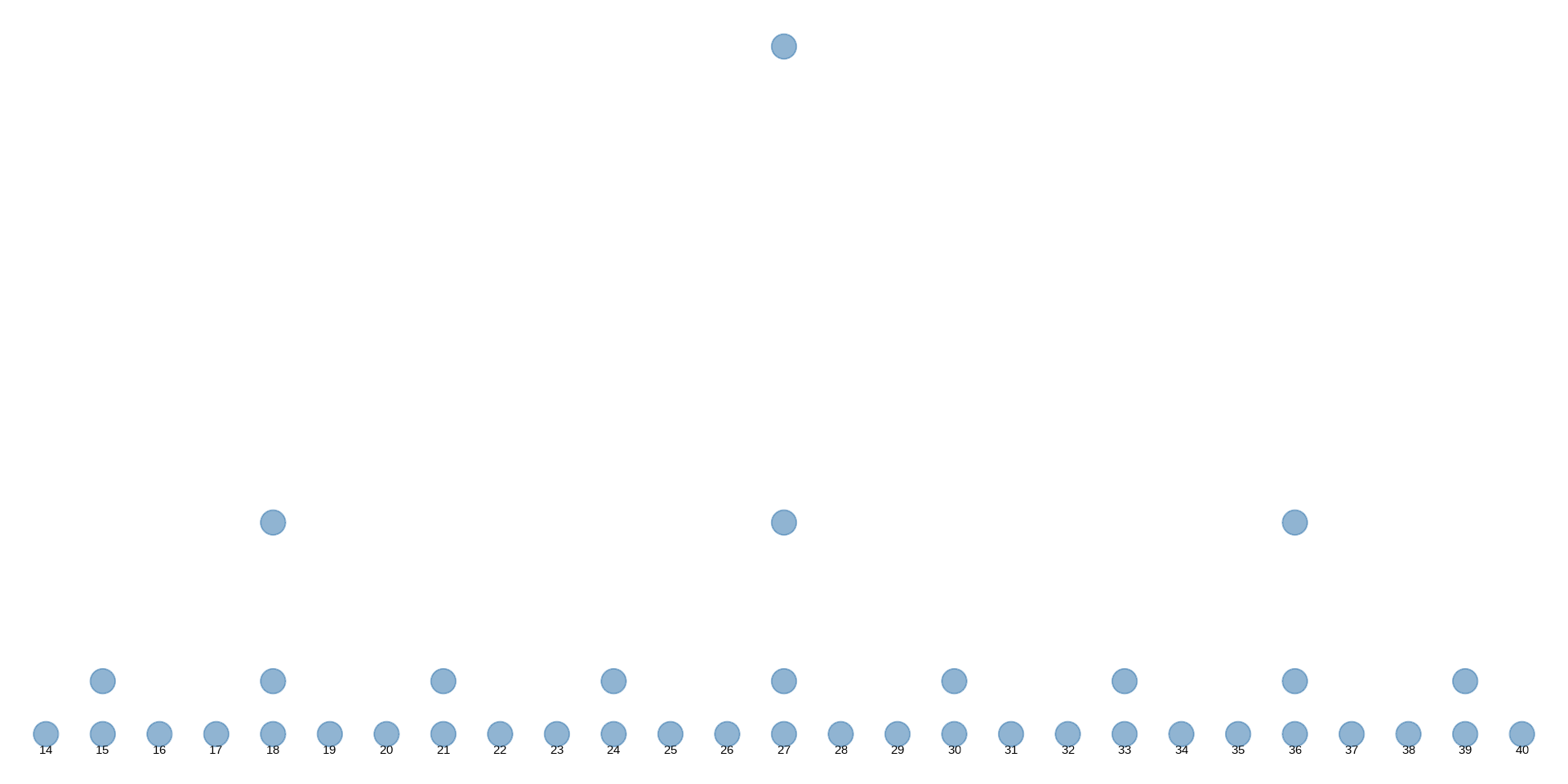
The tree graph (as an igraph object) can be converted to a phylo object using as.phylo() method provided in the treeio package (Table Table 7.1). The ggtree supports directly visualizing tree graph as demonstrated in Figure Figure 7.6. Note that currently not all igraph objects can be supported by ggtree. Currently, it can only be supported when it is a tree graph.
library(igraph)g <-graph.tree(40, 3)
Warning: `graph.tree()` was deprecated in igraph 2.1.0.
ℹ Please use `make_tree()` instead.
Warning: Computation failed in `stat_tree()`.
Caused by error in `dplyr::filter()`:
ℹ In argument: `.data$node != .rootnode.tbl_tree(df)$node`.
Caused by error:
! invalid tbl_tree object.
  missing column:
    label.
Figure 7.6: Visualizing a tree graph. The lines with arrows indicate the relationship between the parent node and the child node. All nodes were indicated by steelblue circle points.
7.5 Other Tree-like Structures
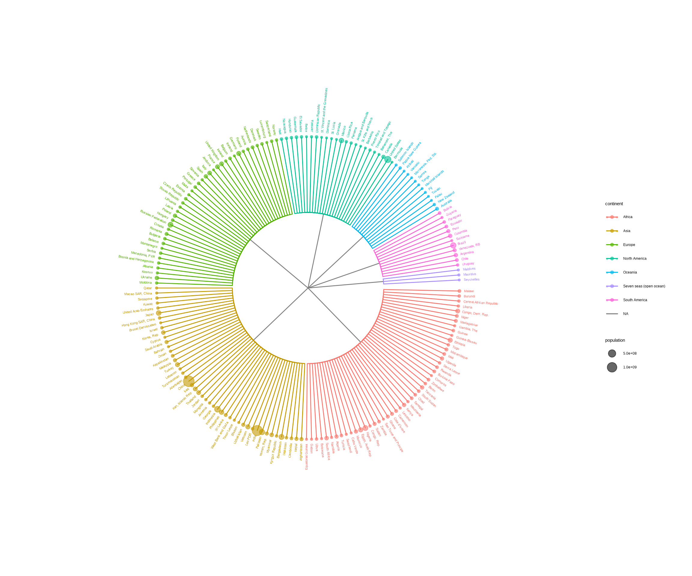
The ggtree package can be used to visualize any data in a hierarchical structure. Here, we use the GNI (Gross National Income) numbers in 2014 as an example. After preparing an edge list, that is a matrix or data frame that contains two columns indicating the relationship of parent and child nodes, we can use the as.phylo() method provided by the treeio package to convert the edge list to a phylo object. Then it can be visualized using ggtree with associated data. In this example, the population was used to scale the size of circle points for each country (Figure Figure 7.7).
Figure 7.7: Visualizing data in any hierarchical structure. Hierarchical data represented as nodes connected by edges can be converted to a phylo object and visualized by r Biocpkg("ggtree") to explore their relationships or other properties that are associated with the relationships.
7.6 Summary
The ggtree supports various tree objects defined in the R language and extension packages, which makes it very easy to integrate ggtree into existing pipelines. Moreover, ggtree allows external data integration and exploration of these data on the tree, which will greatly promote the data visualization and result in interpretation in the downstream analysis of existing pipelines. Most importantly, the support for converting edge list to a tree object enables more tree-like structures to be incorporated into the framework of treeio and ggtree. This will enable more tree-like structures and related heterogeneous data in different disciplines to be integrated and visualized through treeio and ggtree, which facilitates integrated analysis and comparative analysis to discover more systematic patterns and insights.
Callahan, B. J., McMurdie, P. J., Rosen, M. J., Han, A. W., Johnson, A. J. A., & Holmes, S. P. (2016). DADA2: High-resolution sample inference from Illumina amplicon data. Nature Methods, 13(7), 581–583. https://doi.org/10.1038/nmeth.3869
Kuczynski, J., Stombaugh, J., Walters, W. A., González, A., Caporaso, J. G., & Knight, R. (2011). Using QIIME to analyze 16S rRNA gene sequences from MicrobialCommunities. Current Protocols in Bioinformatics / Editoral Board, Andreas D. Baxevanis ... [Et Al.], CHAPTER, Unit10.7. https://doi.org/10.1002/0471250953.bi1007s36
Kunin, V., & Hugenholtz, P. (2010). PyroTagger : A fast , accurate pipeline for analysis of rRNA amplicon pyrosequence data. The Open Journal, 1–8. http://www.theopenjournal.org/toj_articles/1
Schloss, P. D., Westcott, S. L., Ryabin, T., Hall, J. R., Hartmann, M., Hollister, E. B., Lesniewski, R. A., Oakley, B. B., Parks, D. H., Robinson, C. J., Sahl, J. W., Stres, B., Thallinger, G. G., Van Horn, D. J., & Weber, C. F. (2009). Introducing mothur: Open-source, platform-independent, community-supported software for describing and comparing microbial communities. Applied and Environmental Microbiology, 75(23), 7537–7541. https://doi.org/10.1128/AEM.01541-09
Wang, L.-G., Lam, T. T.-Y., Xu, S., Dai, Z., Zhou, L., Feng, T., Guo, P., Dunn, C. W., Jones, B. R., Bradley, T., Zhu, H., Guan, Y., Jiang, Y., & Yu, G. (2020). Treeio: An r package for phylogenetic tree input and output with richly annotated and associated data. Molecular Biology and Evolution, 37(2), 599–603. https://doi.org/10.1093/molbev/msz240
Yu, G. (2020). Using ggtree to visualize data on tree-like structures. Current Protocols in Bioinformatics, 69(1), e96. https://doi.org/10.1002/cpbi.96
Yu, G., Lam, T. T.-Y., Zhu, H., & Guan, Y. (2018). Two methods for mapping and visualizing associated data on phylogeny using ggtree. Molecular Biology and Evolution, 35(12), 3041–3043. https://doi.org/10.1093/molbev/msy194
Yu, G., Smith, D. K., Zhu, H., Guan, Y., & Lam, T. T.-Y. (2017). Ggtree: An r package for visualization and annotation of phylogenetic trees with their covariates and other associated data. Methods in Ecology and Evolution, 8(1), 28–36. https://doi.org/10.1111/2041-210X.12628