Trees are one of the most fundamental data structures for representing hierarchical relationships. Although this book uses phylogenetic trees as its primary running example — they are where the ggtree package suite was born and where its richest applications live — the suite itself is not tied to evolutionary biology. Any data that can be organized as a set of nodes connected by parent-child edges can be imported, manipulated, and visualized with the tools introduced in this book. Hierarchical clustering dendrograms, taxonomic classifications, directory trees, and the tree-shaped subgraphs of general graphs are all first-class citizens.
The tree data model
Whatever their origin, all trees share the same three ingredients:
- Nodes: external nodes (tips/leaves) and internal nodes. In evolutionary biology, tips represent sampled taxa and internal nodes represent hypothetical ancestors; in a clustering dendrogram, tips represent observations and internal nodes represent clusters; in a directory tree, tips are files and internal nodes are folders.
- Edges: the parent-child links between nodes, optionally associated with a length (genetic divergence in a phylogeny, fusion height in a dendrogram, file size in a directory tree).
- Associated data: any additional variables attached to nodes or branches — bootstrap support, sample metadata, cluster statistics, etc.
The tidytree package (Chapter @ref(sec-chapter2)) represents these ingredients as a tidy data frame of nodes with their positions, parent, branch length, and any associated data, so that the dplyr verbs can be used to manipulate trees of any origin. The treeio package (Chapter @ref(chapter1)) provides parsers and converters that bring different tree sources into this model, and ggtree (Chapter @ref(sec-chapter4)) visualizes it with the ggplot2 grammar of graphics.
Trees across disciplines
Table Table 1.1 summarizes common tree types, how they typically arise in R, and where they are covered in this book.
If your data fits any row of this table, the rest of this book applies to you. Readers from outside evolutionary biology can skim the phylogenetics-specific passages — they are marked with domain notes such as the one below — and follow the general workflow: import (Part I) → visualize (Part II) → extend (Part III).
Phylogenetic trees: a domain perspective
This section introduces concepts from evolutionary biology — taxa, ancestors, bootstrap support, substitution models — that are specific to phylogenetic trees. Readers working with dendrograms, taxonomies, or other tree-like structures can jump directly to Chapter @ref(chapter1); the tree formats described there are used well beyond phylogenetics.
Overview of Phylogenetic Tree Construction
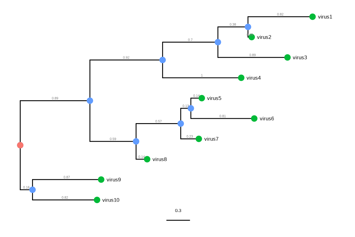
Phylogenetic trees are used to describe genealogical relationships among a group of organisms, which can be constructed based on the genetic sequences of the organisms. A rooted phylogenetic tree represents a model of evolutionary history depicted by ancestor-descendant relationships between tree nodes and clustering of ‘sister’ or ‘cousin’ organisms at a different level of relatedness, as illustrated in Figure Figure 1.1. In infectious disease research, phylogenetic trees are usually built from the pathogens’ gene or genome sequences to show which pathogen sample is genetically closer to another sample, providing insights into the underlying unobserved epidemiologic linkage and the potential source of an outbreak.
(ref:phylogenyscap) Components of a phylogenetic tree.
(ref:phylogenycap) Components of a phylogenetic tree. External nodes (green circles), also called ‘tips’, represent actual organisms sampled and sequenced (e.g., viruses in infectious disease research). They are the ‘taxa’ in the terminology of evolutionary biology. The internal nodes (blue circles) represent hypothetical ancestors for the tips. The root (red circle) is the common ancestor of all species in the tree. The horizontal lines are branches and represent evolutionary changes (gray number) measured in a unit of time or genetic divergence. The bar at the bottom provides the scale of these branch lengths.
Warning: Using `size` aesthetic for lines was deprecated in ggplot2 3.4.0.
ℹ Please use `linewidth` instead.
ℹ The deprecated feature was likely used in the ggtree package.
  Please report the issue at <https://github.com/YuLab-SMU/ggtree/issues>.
A phylogenetic tree can be constructed from genetic sequences using distance-based methods or character-based methods. Distance-based methods, including the unweighted pair group method with arithmetic means (UPGMA) and the Neighbor-joining (NJ), are based on the matrix of pairwise genetic distances calculated between sequences. The character-based methods, including maximum parsimony (MP) (Fitch, 1971), maximum likelihood (ML) (Felsenstein, 1981), and Bayesian Markov Chain Monte Carlo (BMCMC) method (Rannala & Yang, 1996), are based on a mathematical model that describes the evolution of genetic characters and searches for the best phylogenetic tree according to their optimality criteria.
The MP method assumes that the evolutionary change is rare and minimizes the amount of character-state changes (e.g., number of DNA substitutions). The criterion is similar to Occam’s razor, that the simplest hypothesis that can explain the data is the best hypothesis. Unweighted parsimony assumes mutations across different characters (nucleotides or amino acids) are equally likely, while the weighted method assumes the unequal likelihood of mutations (e.g., the third codon position is more liable than other codon positions; and the transition mutations have a higher frequency than transversion). The concept of the MP method is straightforward and intuitive, which is a probable reason for its popularity amongst biologists who care more about the research question rather than the computational details of the analysis. However, this method has several disadvantages, in particular, the tree inference can be biased by the well-known systematic error called long-branch attraction (LBA) that incorrectly infer distantly related lineages as closely related (Felsenstein, 1978). This is because the MP method poorly takes into consideration of many sequence evolution factors (e.g., reversals and convergence) that are hardly observable from the existing genetic data.
The maximum likelihood (ML) method and Bayesian Markov Chain Monte Carlo (BMCMC) method are the two most commonly used methods in phylogenetic tree construction and are most often used in scientific publications. ML and BMCMC methods require a substitution model of sequence evolution. Different sequence data have different substitution models to formulate the evolutionary process of DNA, codon and amino acid. There are several models for nucleotide substitution, including JC69, K2P, F81, HKY, and GTR (Arenas, 2015). These models can be used in conjunction with the rate variation across sites (denoted as +\(\Gamma\))) (Yang, 1994) and the proportion of invariable sites (denoted as +I) (Shoemaker & Fitch, 1989). Previous research (Lemmon & Moriarty, 2004) had suggested that misspecification of substitution model might bias phylogenetic inference. Procedural testing for the best-fit substitution model is recommended.
The optimal criterion of the ML method is to find the tree that maximizes the likelihood given the sequence data. The procedure of the ML method is simple: calculating the likelihood of a tree and optimizing its topology and branches (and the substitution model parameters, if not fixed) until the best tree is found. Heuristic search, such as those implemented in PhyML and RAxML, is often used to find the best tree based on the likelihood criterion. The Bayesian method finds the tree that maximizes posterior probability by sampling trees through MCMC based on the given substitution model. One of the advantages of BMCMC is that parameter variance and tree topological uncertainty, included by the posterior clade probability, can be naturally and conveniently obtained from the sampling trees in the MCMC process. Moreover, the influence of topological uncertainty on other parameter estimates is also naturally integrated into the BMCMC phylogenetic framework.
In a simple phylogenetic tree, data associated with the tree branches/nodes could be the branch lengths (indicating genetic or time divergence) and lineage supports such as bootstrap values estimated from bootstrapping procedure or posterior clade probability summarized from the sampled trees in the BMCMC analysis.
Arenas, M. (2015). Trends in substitution models of molecular evolution.
Frontiers in Genetics,
6.
https://doi.org/10.3389/fgene.2015.00319
Felsenstein, J. (1978). Cases in which
Parsimony or
Compatibility Methods will be
Positively Misleading.
Systematic Biology,
27(4), 401–410.
https://doi.org/10.1093/sysbio/27.4.401
Felsenstein, J. (1981).
Evolutionary trees from DNA sequences: A maximum likelihood approach.
Journal of Molecular Evolution,
17(6), 368–376.
Fitch, W. M. (1971). Toward
Defining the
Course of
Evolution:
Minimum Change for a
Specific Tree Topology.
Systematic Zoology,
20(4), 406–416.
https://doi.org/10.2307/2412116
Lemmon, A. R., & Moriarty, E. C. (2004). The importance of proper model assumption in bayesian phylogenetics.
Systematic Biology,
53(2), 265–277.
https://doi.org/10.1080/10635150490423520