3 Spatial statistical analysis
SVP implements several spatial statistical algorithms to explore the spatial distribution of cell function or other features from three aspects: whether cell function states have spatial variability, where spatially variable cell functions cluster, and the co-distribution patterns of spatially variable cell functions with other features. The following sections provide a detailed description of each aspect.
3.1 Univariate spatial statistical analysis
This section addresses whether the feature is spatially variable and identifies its high-cluster areas. In detail, to identify the spatial variable features, SVP implements three spatial autocorrelation algorithms using Rcpp and RcppParallel: global Moran’s I, Geary’s C and Getis-Ord’s G. To identify the spatial high-cluster areas, SVP implements two local univariate spatial statistical algorithms using Rcpp and RcppParallel: local Getis-Ord’s G and local Moran’s I.
3.1.1 Identification of spatial variable features
Here, we identify the spatial variable cell-types using runDetectSVG, which implements the global Moran’s I, Geary’s C and Getis-Ord’s G algorithms.
# First approach:
# we can first obtain the target gsvaExp with gsvaExp names via
# gsvaExp() function, for example, CellTypeFree
pdac_a_spe |> gsvaExp("CellTypeFree")
#> class: SpatialExperiment
#> dim: 20 428
#> metadata(0):
#> assays(1): affi.score
#> rownames(20): Acinar_cells Ductal_terminal_ductal_like ... RBCs
#>   Fibroblasts
#> rowData names(4): exp.gene.num gset.gene.num gene.occurrence.rate
#>   geneSets
#> colnames(428): Spot1 Spot2 ... Spot427 Spot428
#> colData names(3): cluster_domain sizeFactor sample_id
#> reducedDimNames(0):
#> mainExpName: NULL
#> altExpNames(0):
#> spatialCoords names(2) : x y
#> imgData names(0):

# Then we use runDetectSVG with method = 'moran' to identify the spatial variable
# cell-types with global Moran's I.

celltype_free.I <- pdac_a_spe |> gsvaExp("CellTypeFree") |>
  runDetectSVG(
    assay.type = 'affi.score', # because default is 'logcounts', it should be adjused
    method = 'moransi',
    action = 'only'
  )
#> Identifying the spatially variable gene sets (pathway) based on moransi
#> elapsed time is 0.077000 seconds

celltype_free.I |> dplyr::arrange(rank) |> head()
#>                                            obs expect.moransi sd.moransi
#> Cancer_clone_A                       0.7402441    -0.00234192 0.02807961
#> Cancer_clone_B                       0.7187722    -0.00234192 0.02806609
#> Acinar_cells                         0.6959057    -0.00234192 0.02788079
#> mDCs_A                               0.5823319    -0.00234192 0.02760418
#> Ductal_CRISP3_high-centroacinar_like 0.5605952    -0.00234192 0.02794187
#> Endothelial_cells                    0.5362277    -0.00234192 0.02757573
#>                                      Z.moransi        pvalue          padj rank
#> Cancer_clone_A                        26.44573 2.042568e-154 4.085135e-153    1
#> Cancer_clone_B                        25.69343 6.921386e-146 6.921386e-145    2
#> Acinar_cells                          25.04404 1.013736e-138 6.758238e-138    3
#> mDCs_A                                21.18062 7.205485e-100  3.602743e-99    4
#> Ductal_CRISP3_high-centroacinar_like  20.14672  1.437699e-90  5.750794e-90    5
#> Endothelial_cells                     19.53057  3.018138e-85  1.006046e-84    6

# Second approach:
# the result was added to the original object by specific the
# gsvaexp argument in the runDetectSVG
pdac_a_spe <- pdac_a_spe |>
  runDetectSVG(
    gsvaexp = 'CellTypeFree',
    method = 'moran'
    )
#> The `gsvaexp` was specified, the specified `gsvaExp` will be used to detect 'svg'.
#> Identifying the spatially variable gene sets (pathway) based on moransi
#> elapsed time is 0.064000 seconds
#> The result is added to the input object, which can be extracted using
#> `svDf()` with type='sv.moransi' for `SingleCellExperiment` or `SpatialExperiment`.
#> If input object is `SVPExperiment`, and `gsvaexp` is specified
#> the result can be extracted by `gsvaExp()` (return a `SingleCellExperiment`
#> or `SpatialExperiment`),then also using `svDf()` to extract.
gsvaExp(pdac_a_spe, 'CellTypeFree') |> svDf("sv.moransi") |> dplyr::arrange(rank) |> head()
#>                                            obs expect.moransi sd.moransi
#> Cancer_clone_A                       0.7402441    -0.00234192 0.02807961
#> Cancer_clone_B                       0.7187722    -0.00234192 0.02806609
#> Acinar_cells                         0.6959057    -0.00234192 0.02788079
#> mDCs_A                               0.5823319    -0.00234192 0.02760418
#> Ductal_CRISP3_high-centroacinar_like 0.5605952    -0.00234192 0.02794187
#> Endothelial_cells                    0.5362277    -0.00234192 0.02757573
#>                                      Z.moransi        pvalue          padj rank
#> Cancer_clone_A                        26.44573 2.042568e-154 4.085135e-153    1
#> Cancer_clone_B                        25.69343 6.921386e-146 6.921386e-145    2
#> Acinar_cells                          25.04404 1.013736e-138 6.758238e-138    3
#> mDCs_A                                21.18062 7.205485e-100  3.602743e-99    4
#> Ductal_CRISP3_high-centroacinar_like  20.14672  1.437699e-90  5.750794e-90    5
#> Endothelial_cells                     19.53057  3.018138e-85  1.006046e-84    6
The obs is the Moran’s I, expect.moransi is the expect Moran’s I (E(I)). Moran’s I quantifies the correlation between a single feature at a specific spatial point or region and its neighboring points or regions. Global Moran’s I usually ranges from -1 to 1, Global Moran’s I significantly above E(I) indicate a distinct spatial pattern or spatial clustering, which occurs when neighboring captured locations tend to have similar feature value. Global Moran’s I around E(I) suggest random spatial expression, that is, absence of spatial pattern. Global Moran’s I significantly below E(I) imply a chessboard-like pattern or dispersion.
# using Geary's C
pdac_a_spe <- pdac_a_spe |>
  runDetectSVG(
    gsvaexp = 'CellTypeFree',
    method = 'geary'
  )
#> The `gsvaexp` was specified, the specified `gsvaExp` will be used to detect 'svg'.
#> Identifying the spatially variable gene sets (pathway) based on gearysc
#> elapsed time is 0.031000 seconds
#> The result is added to the input object, which can be extracted using
#> `svDf()` with type='sv.gearysc' for `SingleCellExperiment` or `SpatialExperiment`.
#> If input object is `SVPExperiment`, and `gsvaexp` is specified
#> the result can be extracted by `gsvaExp()` (return a `SingleCellExperiment`
#> or `SpatialExperiment`),then also using `svDf()` to extract.

gsvaExp(pdac_a_spe, "CellTypeFree") |> svDf('sv.gearysc') |> dplyr::arrange(rank) |> head()
#>                                            obs expect.gearysc sd.gearysc
#> Cancer_clone_A                       0.2709051              1 0.02873561
#> Cancer_clone_B                       0.2880919              1 0.02879022
#> Acinar_cells                         0.3055211              1 0.02952587
#> Ductal_CRISP3_high-centroacinar_like 0.4213014              1 0.02928596
#> mDCs_A                               0.4603825              1 0.03058249
#> Endothelial_cells                    0.4843175              1 0.03068854
#>                                      Z.gearysc        pvalue          padj rank
#> Cancer_clone_A                        25.37252 2.535621e-142 5.071243e-141    1
#> Cancer_clone_B                        24.72743 2.711724e-135 2.711724e-134    2
#> Acinar_cells                          23.52103 1.242716e-122 8.284772e-122    3
#> Ductal_CRISP3_high-centroacinar_like  19.76027  3.272367e-87  1.636183e-86    4
#> mDCs_A                                17.64466  5.592678e-70  2.237071e-69    5
#> Endothelial_cells                     16.80375  1.145504e-63  3.818347e-63    6
The obs is the Geary’s C. Global Geary’s C is another popular index of global spatial autocorrelation, but focuses more on differences between neighboring values. Global Geary’s C usually range from 0 to 2. Global Geary’s C significantly below E[C]=1 indicate a distinct spatial pattern or spatial clustering, the value significantly above E[C]=1 suggest a chessboard-like pattern or dispersion, the value around E[C]=1 imply absence of spatial pattern.
# using Getis-ord's G
pdac_a_spe <- pdac_a_spe |>
  runDetectSVG(
    gsvaexp = 'CellTypeFree',
    method = 'getis'
  )
#> The `gsvaexp` was specified, the specified `gsvaExp` will be used to detect 'svg'.
#> Identifying the spatially variable gene sets (pathway) based on getisord
#> elapsed time is 0.030000 seconds
#> The result is added to the input object, which can be extracted using
#> `svDf()` with type='sv.getisord' for `SingleCellExperiment` or `SpatialExperiment`.
#> If input object is `SVPExperiment`, and `gsvaexp` is specified
#> the result can be extracted by `gsvaExp()` (return a `SingleCellExperiment`
#> or `SpatialExperiment`),then also using `svDf()` to extract.

gsvaExp(pdac_a_spe, "CellTypeFree") |> svDf('sv.getisord') |> dplyr::arrange(rank) |> head()
#>                                              obs   expect.G         sd.G
#> Cancer_clone_A                       0.007214987 0.00234192 0.0001844816
#> Cancer_clone_B                       0.007406175 0.00234192 0.0001975938
#> Acinar_cells                         0.007109879 0.00234192 0.0001920919
#> mDCs_A                               0.005853463 0.00234192 0.0001651428
#> Ductal_CRISP3_high-centroacinar_like 0.005800695 0.00234192 0.0001749367
#> Endothelial_cells                    0.005749155 0.00234192 0.0001750884
#>                                           Z.G        pvalue          padj rank
#> Cancer_clone_A                       26.41492 4.617621e-154 9.235241e-153    1
#> Cancer_clone_B                       25.62962 3.567592e-145 3.567592e-144    2
#> Acinar_cells                         24.82124 2.644298e-136 1.762865e-135    3
#> mDCs_A                               21.26368 1.231569e-100 6.157844e-100    4
#> Ductal_CRISP3_high-centroacinar_like 19.77158  2.615753e-87  1.046301e-86    5
#> Endothelial_cells                    19.46009  1.196819e-84  3.989397e-84    6
The obs is the Getis-Ord’s G of each cell-type. Global Getis-Ord’s G measures global spatial autocorrelation by evaluating the clustering of high/low value, specifically identifying hot spots or cold spots. Global Getis-Ord’s G values have no fixed range, as they depend on the specific dataset and spatial weight matrix. Global Getis-Ord’s G significantly above E(G) indicate a distinct spatial pattern or spatial clustering, which occurs when neighboring captured locations tend to have similar feature value. Global Getis-Ord’s G around E(G) suggest random spatial expression, that is, absence of spatial pattern. Global Getis-Ord’s G significantly below E(G) imply a chessboard-like pattern or dispersion.
So the Cancer clone A, Cancer clone B, and Acinar cells were more concentrated in the spatial distribution compare to others.
3.1.2 Identification of local spatial aggregation areas
Next, we can identify the spatial high-cluster areas for the spatial variable features via runLISA, which provides two local spatial statistics algorithms: Local Getis-Ord’s G and Local Moran’s I
celltypefree_lisares <- pdac_a_spe |>
   gsvaExp("CellTypeFree") %>%
   runLISA(features=rownames(.), assay.type=1)

celltypefree_lisares$Cancer_clone_A |> head()
#>                 Gi       E.Gi       Var.Gi      Z.Gi Pr (z != E(Gi))
#> Spot1 0.0001746202 0.00234192 1.649943e-06 -1.687270      0.09155141
#> Spot2 0.0003158584 0.00234192 2.996272e-06 -1.170475      0.24180992
#> Spot3 0.0002774819 0.00234192 2.489785e-06 -1.308341      0.19075761
#> Spot4 0.0001673520 0.00234192 2.489501e-06 -1.378215      0.16813699
#> Spot5 0.0004016950 0.00234192 2.994463e-06 -1.121225      0.26219219
#> Spot6 0.0004403359 0.00234192 2.130895e-06 -1.302670      0.19268729
#>       cluster.no.test cluster.test
#> Spot1             Low       NoSign
#> Spot2             Low       NoSign
#> Spot3             Low       NoSign
#> Spot4             Low       NoSign
#> Spot5             Low       NoSign
#> Spot6             Low       NoSign
Local Getis-Ord’s G (Gi) measures the aggregation of a feature value in a specific spot and its neighbors, determining if locations are significantly clustered with high (hot spots) or low values (cold spots). Gi usually have no fixed range, a larger Gi indicates a stronger clustering of high expression for the feature in captured location and its neighboring spots, while a smaller Gi indicates a stronger clustering of low expression.
gsvaExp(pdac_a_spe, 'CellTypeFree') |>
  plot_lisa_feature(
    lisa.res = celltypefree_lisares[c('Cancer_clone_A', 'Cancer_clone_B', 'Acinar_cells')],
    assay.type = 1,
    gap_line_width = .18
  )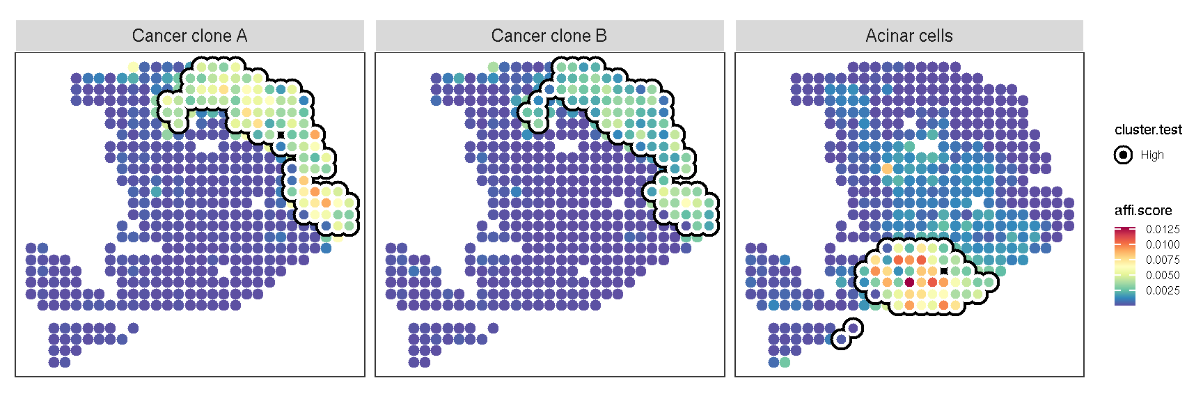
Figure 3.1: The result of local Getis-Ord for cell-type
The highlighted area signifies that the feature is significantly clustered in this region.
We also can use local Moran’s I method to identify the region.
celltypefree_lisa.i <- pdac_a_spe |>
   gsvaExp("CellTypeFree") %>%
   runLISA(
     features = rownames(.),
     assay.type = 1,
     method = 'localmoran'
   )

celltypefree_lisa.i$Cancer_clone_A |> head()
#>              Ii          E.Ii     Var.Ii     Z.Ii Pr (z != E(Ii))
#> Spot1 0.2411323 -0.0004394871 0.02049855 1.687270      0.09155141
#> Spot2 0.2610045 -0.0005894003 0.04994947 1.170475      0.24180992
#> Spot3 0.2907443 -0.0007044064 0.04962291 1.308341      0.19075761
#> Spot4 0.3124376 -0.0007329623 0.05163310 1.378215      0.16813699
#> Spot5 0.2792327 -0.0007358277 0.06234951 1.121225      0.26219219
#> Spot6 0.2256567 -0.0005002450 0.03014053 1.302670      0.19268729
#>       cluster.no.test cluster.test
#> Spot1         Low-Low       NoSign
#> Spot2         Low-Low       NoSign
#> Spot3         Low-Low       NoSign
#> Spot4         Low-Low       NoSign
#> Spot5         Low-Low       NoSign
#> Spot6         Low-Low       NoSign
Local Moran’s I (Ii) measures the spatial correlation between a feature’s values in a specific area and its neighbors, assessing the similarity or difference between a location’s value and those of its surroundings. Ii also have no fixed range, a larger Ii signifies a stronger positive correlation in a region and its neighbors, with clusters of high or low values. A smaller value indicates a negative correlation, where high values are next to low values, or vice versa.
gsvaExp(pdac_a_spe, "CellTypeFree") |>
  plot_lisa_feature(
     lisa.res = celltypefree_lisa.i[c('Cancer_clone_A', 'Cancer_clone_B', 'Acinar_cells')],
     clustertype = 'High-High',
     assay.type = 1,
     gap_line_width = .18
  )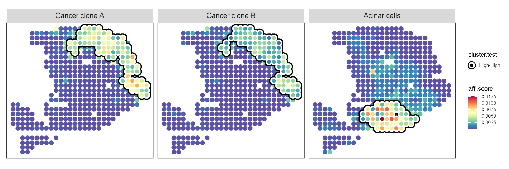
Figure 3.2: The result of local Moran for cell-type
3.2 Bivariate spatial statistical analysis
Next, to explore the bivariate spatial co-distribution, SVP implements global and local bivariate spatial statistics algorithms. Global bivariate spatial statistics algorithm can be used to identify whether the bivariate is co-cluster in the specific space. Local bivariate spatial algorithm is to find the areas of spatial co-clustering of bivariate.
3.2.1 Global bivariate spatial analysis
Here, we use runGLOBALBV of SVP to explore the spatial co-distribution between the cell-types.
gbv.res <- pdac_a_spe |>
  gsvaExp('CellTypeFree') |>
  runGLOBALBV(
    features1 = names(markerList),
    assay.type = 1,
    permutation = NULL, # if permutation is NULL, mantel test will be used to calculated the pvalue
    add.pvalue = TRUE,
    alternative = 'greater' # one-side test
  )

# gbv.res is a list contained Lee and pvalue matrix.
gbv.res |> as_tbl_df(diag=FALSE, flag.clust = TRUE) |>
  dplyr::filter(grepl("Cancer", x)) |> dplyr::arrange(desc(Lee))
#> # A tibble: 35 × 4
#>    x              y                        Lee   pvalue
#>    <fct>          <fct>                  <dbl>    <dbl>
#>  1 Cancer_clone_A Cancer_clone_B      0.728    0
#>  2 Cancer_clone_B Fibroblasts         0.185    2.04e-27
#>  3 Cancer_clone_A Fibroblasts         0.180    5.82e-27
#>  4 Cancer_clone_B Endothelial_cells   0.000286 4.99e- 1
#>  5 Cancer_clone_A Endothelial_cells  -0.0169   8.07e- 1
#>  6 Cancer_clone_B T_cells_&_NK_cells -0.0442   9.97e- 1
#>  7 Cancer_clone_A RBCs               -0.0443   9.80e- 1
#>  8 Cancer_clone_B RBCs               -0.0513   9.91e- 1
#>  9 Cancer_clone_A T_cells_&_NK_cells -0.0696   1.00e+ 0
#> 10 Cancer_clone_B Macrophages_A      -0.0773   1.00e+ 0
#> # ℹ 25 more rows
The Lee value typically ranges from -1 to 1. When the index is closer to 1, it indicates a strong positive spatial association between the two variables, meaning the high-value areas of one variable tend to overlap with the high-value areas of the other, and low-value areas similarly overlap, showing strong spatial consistency. Conversely, if the index is near -1, it suggests a strong negative spatial association, where the high-value areas of one variable tend to overlap with the low-value areas of the other.
We developed a function plot_heatmap_globalbv to visualize the result of global bivariate spatial analysis
# We can also display the result of global univariate spatial analysis
moran.res <- gsvaExp(pdac_a_spe, 'CellTypeFree') |> svDf("sv.moransi")

# The result of local univariate spatial analysis also can be added
lisa.f1.res <- gsvaExp(pdac_a_spe, "CellTypeFree", withColData = TRUE) |>
    cal_lisa_f1(lisa.res = celltypefree_lisares, group.by = 'cluster_domain')

plot_heatmap_globalbv(gbv.res, moran.t=moran.res, lisa.t=lisa.f1.res)
#> Warning in grid.Call.graphics(C_rect, x$x, x$y, x$width, x$height,
#> resolveHJust(x$just, : semi-transparency is not supported on this device:
#> reported only once per page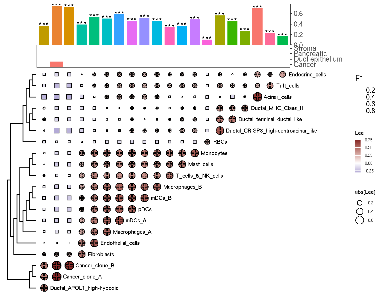
Figure 3.3: The results of clustering analysis of spatial distribution between cell-type
We can explore the spatial co-cluster between the different type of gsvaExp. For example, we explore the spatial co-distribution between the CellTypeFree and CancerSEA of pdac_a_spe object.
# If the number of features is excessive, we recommend selecting
# those with spatial variability.
# celltypeid <- gsvaExp(pdac_a_spe, "CellTypeFree") |> svDf("sv.moransi") |>
#   dplyr::filter(padj<=0.01) |> rownames()
celltypeid <- rownames(gsvaExp(pdac_a_spe, "CellTypeFree"))

cancerseaid <- gsvaExp(pdac_a_spe, "CancerSEA") |>
   runDetectSVG(assay.type = 1, verbose=FALSE) |>
   svDf() |>
   dplyr::filter(padj <= 0.01) |>
   rownames()
#> elapsed time is 0.032000 seconds

runGLOBALBV(
  pdac_a_spe,
  gsvaexp = c("CellTypeFree", "CancerSEA"),
  gsvaexp.features = c(celltypeid, cancerseaid),
  permutation = NULL,
  add.pvalue = TRUE
) -> res.gbv.celltype.cancersea
#> The `gsvaexp` is specified, the specified `gsvaExp` will be
#> used to perform the analysis.

plot_heatmap_globalbv(res.gbv.celltype.cancersea)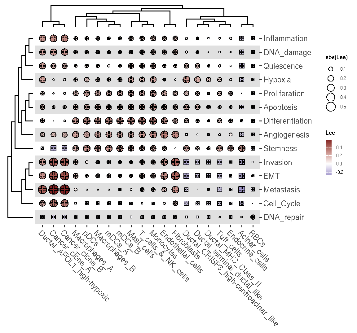
Figure 3.4: The heatmap of spatial correlation between cell tyep and CancerSEA states
3.2.2 Local bivariate spatial analysis
After global bivariate spatial analysis, we found the Cancer cell and Fibroblasts show significant spatial co-aggregation. Next, we use runLOCALBV of SVP to identify the co-aggregation areas.
lbv.res <- pdac_a_spe |>
  gsvaExp('CellTypeFree') |>
  runLOCALBV(features1='Fibroblasts', features2=c('Cancer_clone_A', "Cancer_clone_B"), assay.type=1)

# The result can be added to gsvaExp, then visualized by ggsc.
LISAsce(pdac_a_spe, lisa.res=lbv.res, gsvaexp.name='LBV.res') |>
  gsvaExp("LBV.res") %>%
  plot_lisa_feature(lisa.res = lbv.res, assay.type = 1)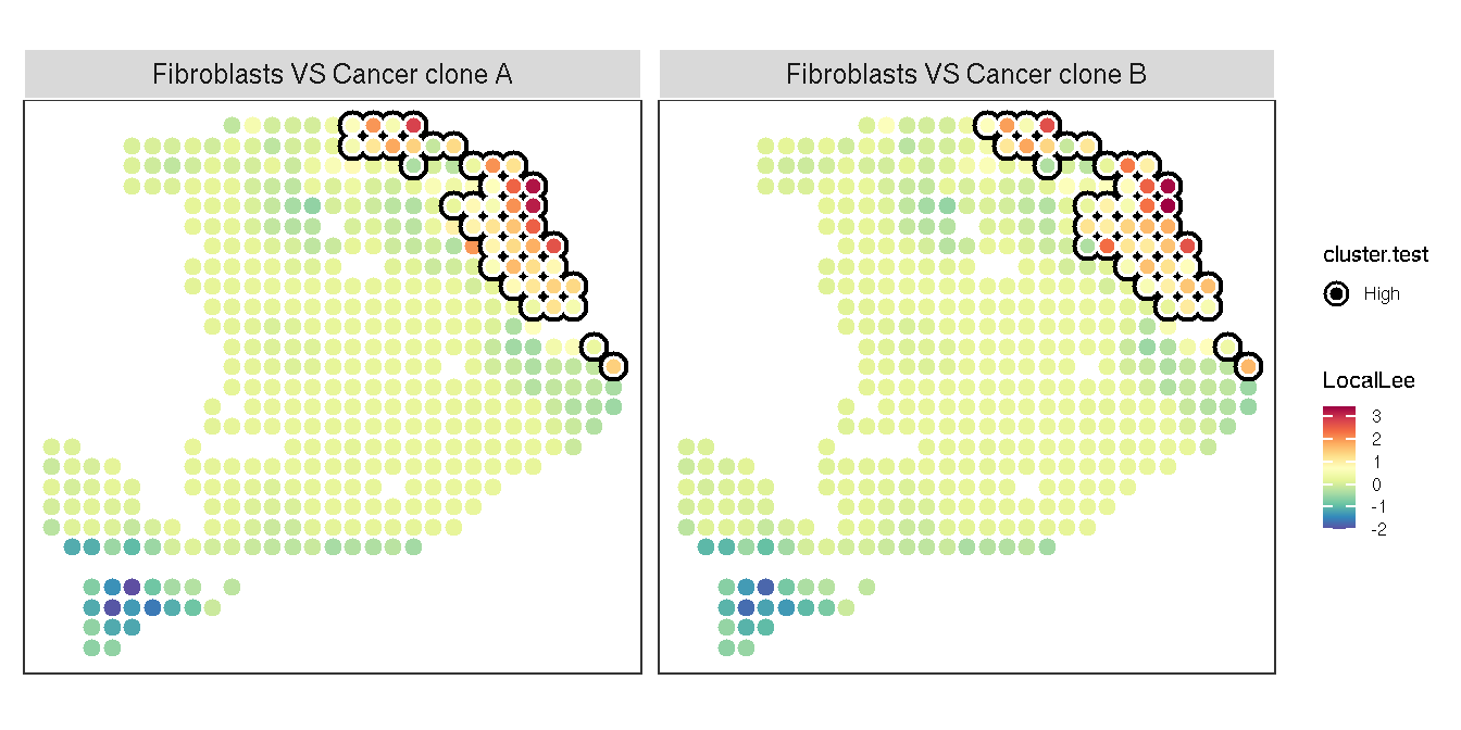
Figure 3.5: The heatmap of Local bivariate spatial analysis
The highlighted area denotes the region where the two variables significantly co-aggregate in space.