2 Quantification of cell states using SVP
SVP can integrate gene or protein lists from existing biomedical databases like cell-type markers (PanglaoDB, CellMarkers), gene ontology (GO), molecular features (MSigDB), and pathways (KEGG, Reactome, Wikipathways), transcription factors, and disease ontology, to assess cell states. Of course, the cell-type markers also can be extracted from reference single cell data. In this vignette, we use the spatial transcriptome and single cell transcriptome of a human pancreatic ductal adenocarcinomas from the article(Moncada et al. 2020) to demonstrate. Here, we first perform the normalization by logNormCounts of scuttle and the MCA dimensionality reduction by runMCA of SVP.
# load the packages required in the vignette
library(SpatialExperiment)
library(SingleCellExperiment)
library(scuttle)
library(scran)
library(SVP)
library(ggsc)
library(ggplot2)
library(magrittr)

# load the spatial transcriptome, it is a SpatialExperiment object
# to build the object, you can refer to the SpatialExperiment package
pdac_a_spe <- readRDS(url("https://raw.githubusercontent.com/xiangpin/Data_for_Vignette_SVP/main/data/pdac_a_spe.rds"))
# we had removed the genes that did not express in any captured location.
# First, we use logNormCounts of scuttle to normalize the spatial transcriptome
pdac_a_spe <- logNormCounts(pdac_a_spe)
# Now the normalized counts was added to the assays of pdac_a_spe as `logcounts`
# it can be extracted via logcounts(pdac_a_spe) or assay(pdac_a_spe, 'logcounts')

# Next, we use `runMCA` of `SVP` to preform the MCA dimensionality reduction
pdac_a_spe <- runMCA(pdac_a_spe, assay.type = 'logcounts')
#> Computing Fuzzy Matrix
#> Computing SVD
#> Computing Coordinates
# The MCA result was added to the reducedDims, it can be extracted by reducedDim(pdac_a_spe, 'MCA')
# more information can refer to SingleCellExperiment package
pdac_a_spe
#> class: SpatialExperiment
#> dim: 13160 428
#> metadata(0):
#> assays(2): counts logcounts
#> rownames(13160): 1-Mar 1-Sep ... ZZEF1 ZZZ3
#> rowData names(0):
#> colnames(428): Spot1 Spot2 ... Spot427 Spot428
#> colData names(3): sample_id cluster_domain sizeFactor
#> reducedDimNames(1): MCA
#> mainExpName: NULL
#> altExpNames(0):
#> spatialCoords names(2) : x y
#> imgData names(1): sample_id
2.1 Quantification of CancerSEA etc function
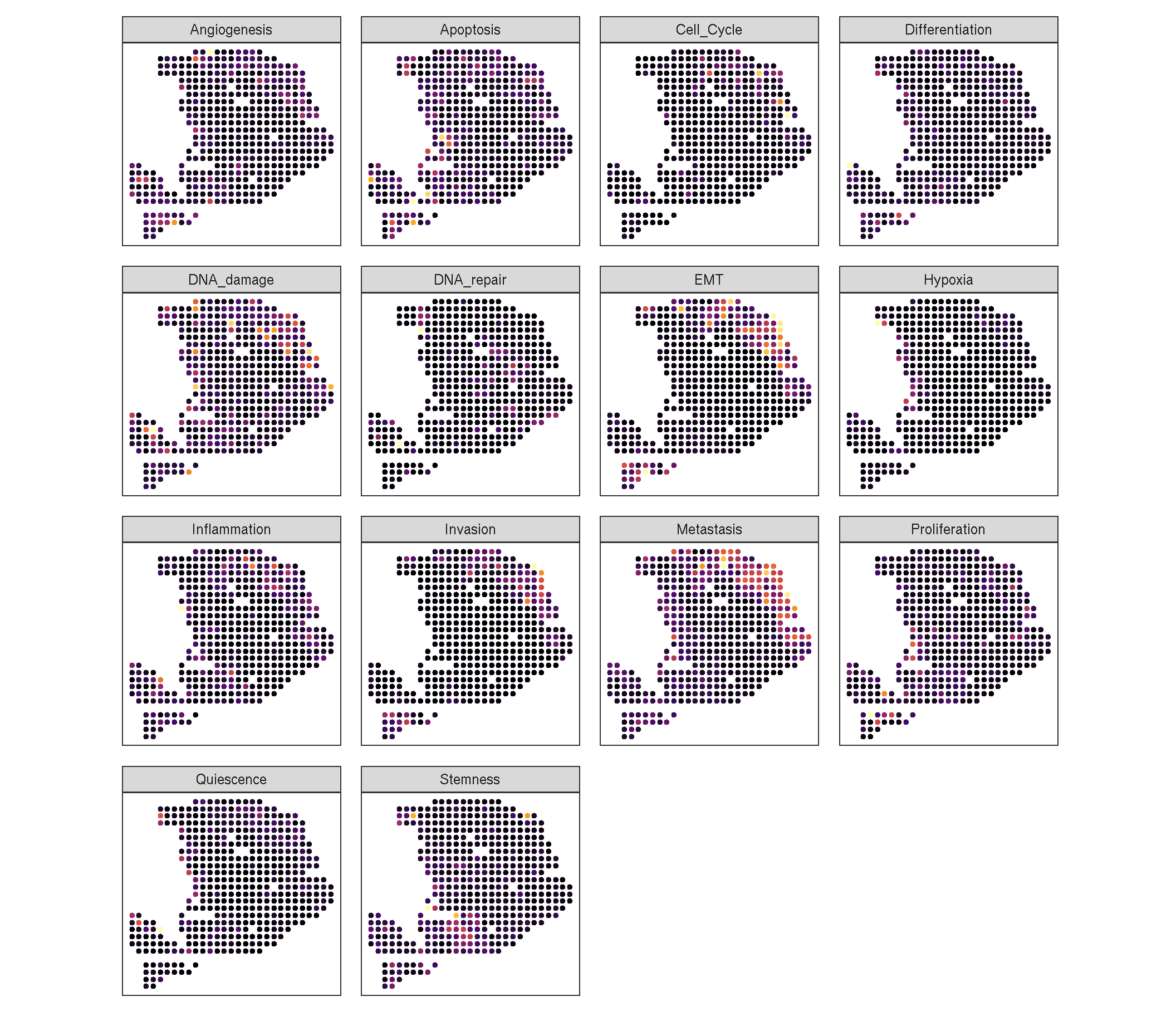
SVP accepts SingleCellExperiment or SpatialExperiment object as input. The gene set should be a named list object, and the elements of the list must be included in the row names of the SingleCellExperiment or SpatialExperiment object. To quantifying the CancerSEA or other function for each captured location, the command runSGSA is used.
# This is gene list of Cancer Single-cell State Atlas to comprehensively decode distinct
# functional states of cancer cells at single cell resolution.
data(CancerSEASymbol)

# It contains 14 types of cancer single-cell state, you can obtain
# more information via ?CancerSEASymbol
names(CancerSEASymbol)
#>  [1] "Angiogenesis"    "Apoptosis"       "Cell_Cycle"      "Differentiation"
#>  [5] "DNA_damage"      "DNA_repair"      "EMT"             "Hypoxia"
#>  [9] "Inflammation"    "Invasion"        "Metastasis"      "Proliferation"
#> [13] "Quiescence"      "Stemness"

pdac_a_spe <- runSGSA(pdac_a_spe,
                      gset.idx.list = CancerSEASymbol, # The target gene set list
                      assay.type = 'logcounts', # The name of assays of gene profiler
                      gsvaExp.name = 'CancerSEA' # The name of result to save to gsvaExps slot
              )
#> Building the nearest neighbor graph with the distance between features and
#> cells ...
#> elapsed time is 3.968000 seconds
#> Building the seed matrix using the gene set and the nearest neighbor graph for
#> random walk with restart ...
#> elapsed time is 0.040000 seconds
#> Calculating the affinity score using random walk with restart ...
#> elapsed time is 0.117000 seconds
#> Tidying the result of random walk with restart ...
#> elapsed time is 0.007000 seconds
#> ORA analysis ...
#> elapsed time is 0.010000 seconds

# Then the result was added to gsvaExps to return a SVPExperiment object, the result
# can be extracted with gsvaExp, you can view more information via help(gsvaExp).
pdac_a_spe
#> class: SVPExperiment
#> dim: 13160 428
#> metadata(0):
#> assays(2): counts logcounts
#> rownames(13160): 1-Mar 1-Sep ... ZZEF1 ZZZ3
#> rowData names(0):
#> colnames(428): Spot1 Spot2 ... Spot427 Spot428
#> colData names(3): sample_id cluster_domain sizeFactor
#> reducedDimNames(1): MCA
#> mainExpName: NULL
#> altExpNames(0):
#> spatialCoords names(2) : x y
#> imgData names(0):
#> gsvaExps names(1) : CancerSEA

gsvaExpNames(pdac_a_spe)
#> [1] "CancerSEA"

# The result is also a SingleCellExperiment or SpatialExperiment.
gsvaExp(pdac_a_spe, 'CancerSEA')
#> class: SpatialExperiment
#> dim: 14 428
#> metadata(0):
#> assays(1): affi.score
#> rownames(14): Angiogenesis Apoptosis ... Quiescence Stemness
#> rowData names(4): exp.gene.num gset.gene.num gene.occurrence.rate
#>   geneSets
#> colnames(428): Spot1 Spot2 ... Spot427 Spot428
#> colData names(3): cluster_domain sizeFactor sample_id
#> reducedDimNames(0):
#> mainExpName: NULL
#> altExpNames(0):
#> spatialCoords names(2) : x y
#> imgData names(0):

# We use sc_spatial of ggsc to visualize the distribution of each functions
# Note: when the number of features is too large, we reco
gsvaExp(pdac_a_spe, 'CancerSEA') %>%
  sc_spatial(
    features = rownames(.),
    mapping = aes(x = x, y = y),
    geom = geom_bgpoint,
    pointsize = 1.2,
    ncol = 4,
    common.legend = FALSE # The output is a patchwork
  ) &
  scale_color_viridis_c(option='B', guide='none')
#> Scale for colour is already present.
#> Adding another scale for colour, which will replace the existing scale.
#> Scale for colour is already present.
#> Adding another scale for colour, which will replace the existing scale.
#> Scale for colour is already present.
#> Adding another scale for colour, which will replace the existing scale.
#> Scale for colour is already present.
#> Adding another scale for colour, which will replace the existing scale.
#> Scale for colour is already present.
#> Adding another scale for colour, which will replace the existing scale.
#> Scale for colour is already present.
#> Adding another scale for colour, which will replace the existing scale.
#> Scale for colour is already present.
#> Adding another scale for colour, which will replace the existing scale.
#> Scale for colour is already present.
#> Adding another scale for colour, which will replace the existing scale.
#> Scale for colour is already present.
#> Adding another scale for colour, which will replace the existing scale.
#> Scale for colour is already present.
#> Adding another scale for colour, which will replace the existing scale.
#> Scale for colour is already present.
#> Adding another scale for colour, which will replace the existing scale.
#> Scale for colour is already present.
#> Adding another scale for colour, which will replace the existing scale.
#> Scale for colour is already present.
#> Adding another scale for colour, which will replace the existing scale.
#> Scale for colour is already present.
#> Adding another scale for colour, which will replace the existing scale.
Figure 2.1: The heatmap of each CancerSEA function
# The other function also can be quantified with runSGSA
# the gset.idx.list supports the named gene list, gson object or
# locate gmt file or html url of gmt.
pdac_a_spe <- runSGSA(
    pdac_a_spe,
    gset.idx.list = "https://data.broadinstitute.org/gsea-msigdb/msigdb/release/2023.2.Hs/h.all.v2023.2.Hs.symbols.gmt",
    gsvaExp.name = 'hallmark',
    assay.type = 'logcounts' # default
)
#> Building the nearest neighbor graph with the distance between features and
#> cells ...
#> elapsed time is 3.566000 seconds
#> Building the seed matrix using the gene set and the nearest neighbor graph for
#> random walk with restart ...
#> elapsed time is 0.026000 seconds
#> Calculating the affinity score using random walk with restart ...
#> elapsed time is 0.206000 seconds
#> Tidying the result of random walk with restart ...
#> elapsed time is 0.012000 seconds
#> ORA analysis ...
#> elapsed time is 0.021000 seconds

# The result also was added to gsvaExps
pdac_a_spe
#> class: SVPExperiment
#> dim: 13160 428
#> metadata(0):
#> assays(2): counts logcounts
#> rownames(13160): 1-Mar 1-Sep ... ZZEF1 ZZZ3
#> rowData names(0):
#> colnames(428): Spot1 Spot2 ... Spot427 Spot428
#> colData names(3): sample_id cluster_domain sizeFactor
#> reducedDimNames(1): MCA
#> mainExpName: NULL
#> altExpNames(0):
#> spatialCoords names(2) : x y
#> imgData names(0):
#> gsvaExps names(2) : CancerSEA hallmark
2.2 Quantification of cell-type
To quantifying the cell-type for each captured location, the gene set should be the marker gene sets of cell-type. It can be the pre-established marker gene sets, such as the markers from CellMarkers or PanglaoDB. High-quality cell marker genes from past reports or your own compilations are acceptable. In addition, It can also be extracted from the reference single cell data. The following sections will detail the specific operations of each approach.
2.2.1 Quantification of cell-type using the pre-established marker gene sets
We can use the pre-established marker gene sets to quantifying the cell-type for each captured location. Here, we used the markers obtained from the CARD, which was used as input for CARDfree command.
# The marker gene sets
load(url("https://github.com/YingMa0107/CARD/blob/master/data/markerList.RData?raw=true"))
markerList |> names()
#>  [1] "Acinar_cells"
#>  [2] "Ductal_terminal_ductal_like"
#>  [3] "Ductal_CRISP3_high-centroacinar_like"
#>  [4] "Cancer_clone_A"
#>  [5] "Ductal_MHC_Class_II"
#>  [6] "Cancer_clone_B"
#>  [7] "mDCs_A"
#>  [8] "Ductal_APOL1_high-hypoxic"
#>  [9] "Tuft_cells"
#> [10] "mDCs_B"
#> [11] "pDCs"
#> [12] "Endocrine_cells"
#> [13] "Endothelial_cells"
#> [14] "Macrophages_A"
#> [15] "Mast_cells"
#> [16] "Macrophages_B"
#> [17] "T_cells_&_NK_cells"
#> [18] "Monocytes"
#> [19] "RBCs"
#> [20] "Fibroblasts"
# We can view the marker gene number of each cell-type.
lapply(markerList, length) |> unlist()
#>                         Acinar_cells          Ductal_terminal_ductal_like
#>                                   49                                   13
#> Ductal_CRISP3_high-centroacinar_like                       Cancer_clone_A
#>                                   34                                   81
#>                  Ductal_MHC_Class_II                       Cancer_clone_B
#>                                    7                                  110
#>                               mDCs_A            Ductal_APOL1_high-hypoxic
#>                                  292                                   47
#>                           Tuft_cells                               mDCs_B
#>                                  128                                  209
#>                                 pDCs                      Endocrine_cells
#>                                  134                                  182
#>                    Endothelial_cells                        Macrophages_A
#>                                  165                                  210
#>                           Mast_cells                        Macrophages_B
#>                                  286                                  167
#>                   T_cells_&_NK_cells                            Monocytes
#>                                   89                                  160
#>                                 RBCs                          Fibroblasts
#>                                   92                                  224

pdac_a_spe <- runSGSA(
                pdac_a_spe,
                gset.idx.list = markerList,
                gsvaExp.name = 'CellTypeFree',
                assay.type = 'logcounts'
              )
#> Building the nearest neighbor graph with the distance between features and
#> cells ...
#> elapsed time is 3.473000 seconds
#> Building the seed matrix using the gene set and the nearest neighbor graph for
#> random walk with restart ...
#> elapsed time is 0.012000 seconds
#> Calculating the affinity score using random walk with restart ...
#> elapsed time is 0.126000 seconds
#> Tidying the result of random walk with restart ...
#> elapsed time is 0.007000 seconds
#> ORA analysis ...
#> elapsed time is 0.011000 seconds

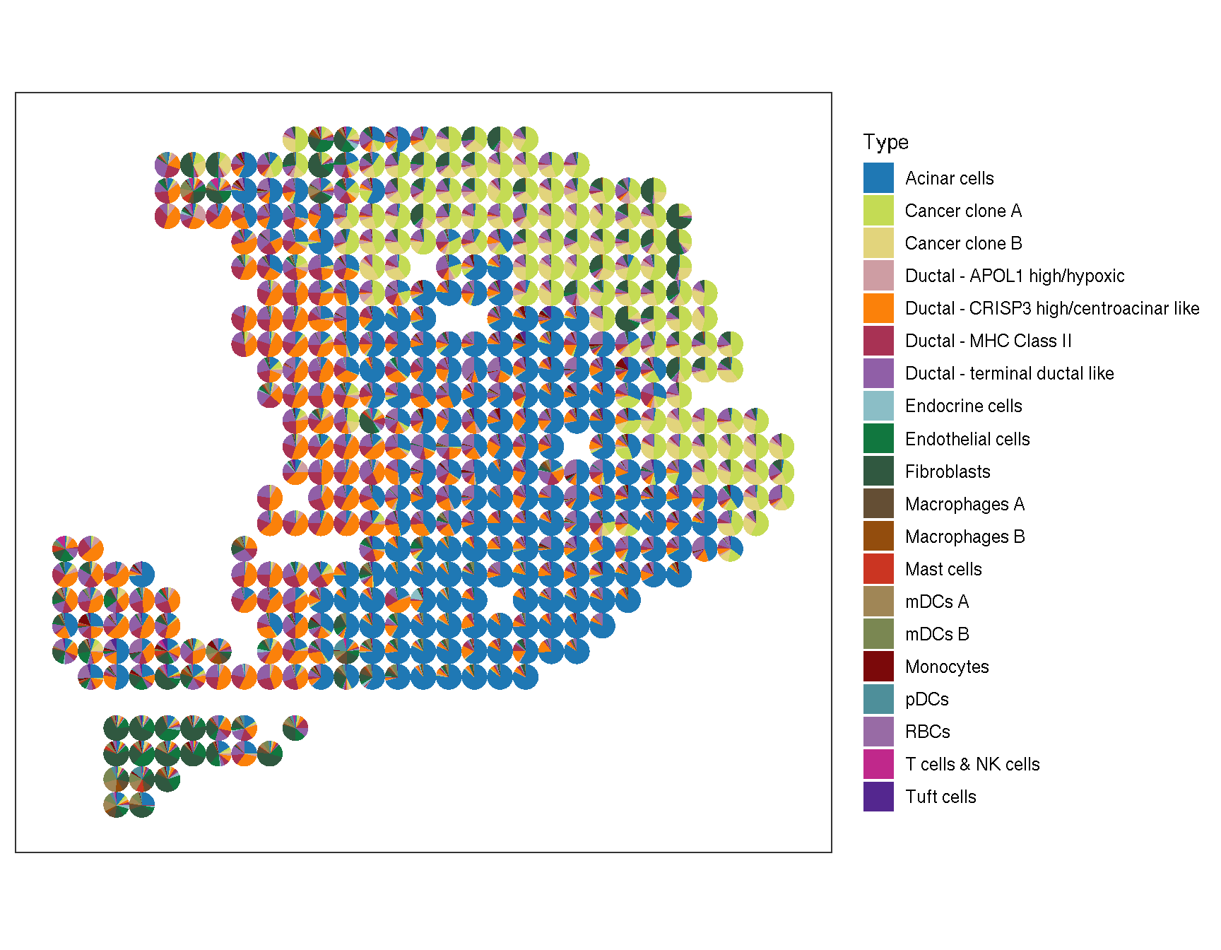
# Then we can visualize the cell-type activity via sc_spatial of SVP with pie plot
gsvaExp(pdac_a_spe, "CellTypeFree") |>
   sc_spatial(
     features = sort(names(markerList)),
     mapping = aes(x = x, y = y),
     plot.pie = TRUE,
     color = NA,
     pie.radius.scale = .9
   )
Figure 2.2: The pie plot of cell-type activity
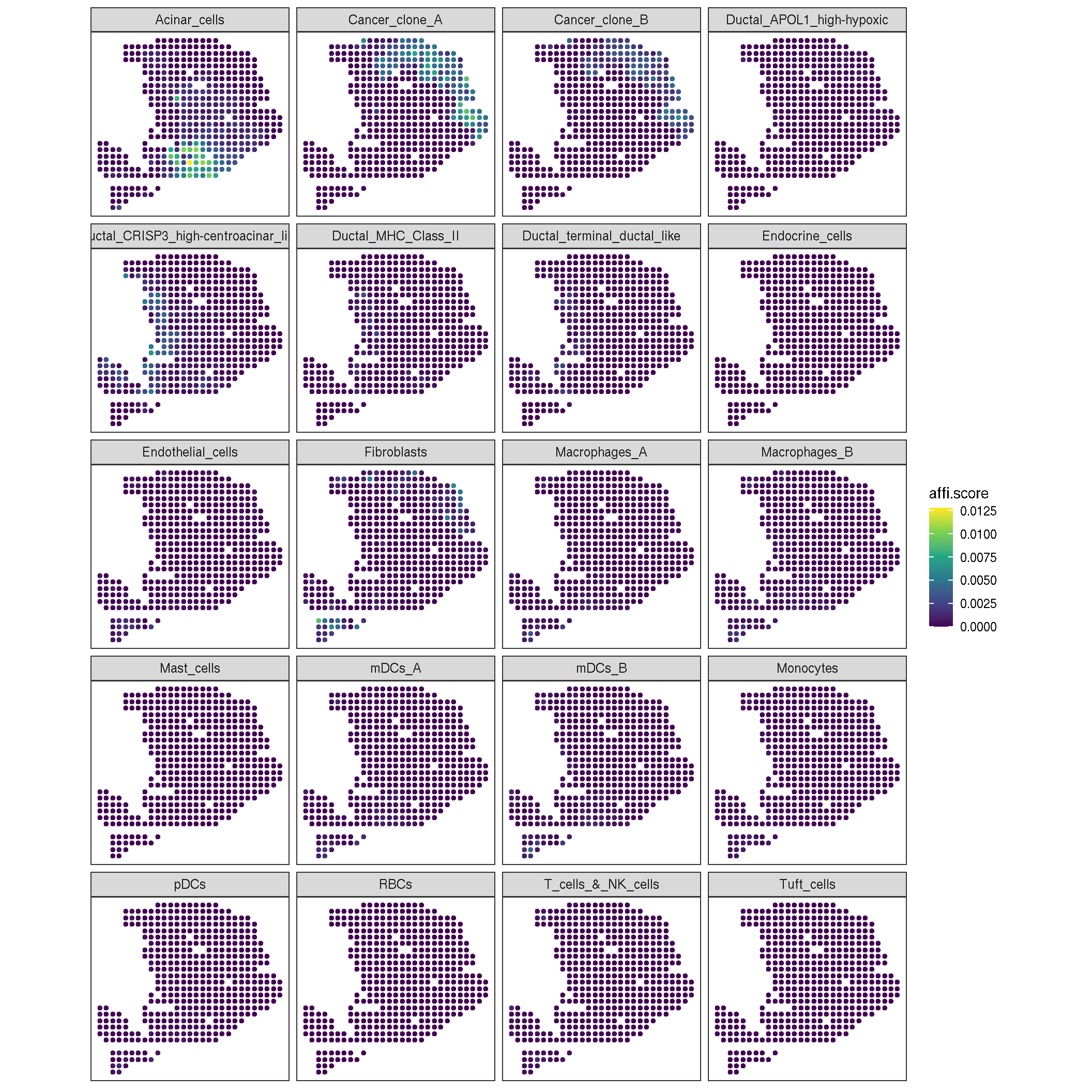
We cal also display each cell-type activity with heat-map according to the spatial coordinate.
pdac_a_spe |> gsvaExp(3) |>
   sc_spatial(
     features = sort(names(markerList)),
     mapping = aes(x = x,  y = y),
     geom = geom_bgpoint,
     pointsize = 1.2,
     ncol = 4
   ) +
   scale_color_viridis_c()
#> Scale for colour is already present.
#> Adding another scale for colour, which will replace the existing scale.
Figure 2.3: the heatmap of each cell-type activity
2.2.2 Quantification of cell-type using the reference single-cell data
This approach requires obtaining the cell-type marker genes from the reference single-cell data. First, the reference single cell data should be normalized. Here, the command of logNormCounts of scuttle is used. Next, the MCA dimensionality reduction is performed by runMCA of SVP. Finally, the marker gene sets of cell-type are extracted via runDetectMarker of SVP.
# load the reference single cell transcriptome
# it is a SingleCellExperiment
pdac_a_sce <- readRDS(url("https://raw.githubusercontent.com/xiangpin/Data_for_Vignette_SVP/main/data/pdac_a_sce.rds"))
pdac_a_sce
#> class: SingleCellExperiment
#> dim: 15418 1926
#> metadata(0):
#> assays(1): counts
#> rownames(15418): 1-Mar 1-Sep ... ZZEF1 ZZZ3
#> rowData names(0):
#> colnames(1926): Cell1 Cell2 ... Cell1925 Cell1926
#> colData names(1): Cell
#> reducedDimNames(0):
#> mainExpName: NULL
#> altExpNames(0):

pdac_a_sce <- logNormCounts(pdac_a_sce)

# obtain the top high variable genes
set.seed(123)
stats <- modelGeneVar(pdac_a_sce)
hvgs <- getTopHVGs(stats)

# perform the MCA reduction.
pdac_a_sce <- pdac_a_sce |> runMCA(assay.type = 'logcounts', subset.row=hvgs[seq(2000)])
#> Computing Fuzzy Matrix
#> Computing SVD
#> Computing Coordinates

# obtain the marker gene sets from reference single-cell transcriptome based on MCA space
refmakergene <- runDetectMarker(pdac_a_sce, group.by='Cell', ntop=200, present.prop.in.group=.2, present.prop.in.sample=.5)
refmakergene |> lapply(length) |> unlist()
#>                           Acinar cells          Ductal - terminal ductal like
#>                                     53                                     82
#> Ductal - CRISP3 high/centroacinar like                         Cancer clone A
#>                                     90                                     90
#>                  Ductal - MHC Class II                         Cancer clone B
#>                                     72                                     90
#>                                 mDCs A            Ductal - APOL1 high/hypoxic
#>                                     89                                     92
#>                             Tuft cells                                 mDCs B
#>                                     87                                     71
#>                                   pDCs                        Endocrine cells
#>                                     50                                     60
#>                      Endothelial cells                          Macrophages A
#>                                     81                                     76
#>                             Mast cells                          Macrophages B
#>                                    120                                     48
#>                     T cells & NK cells                              Monocytes
#>                                     39                                     56
#>                                   RBCs                            Fibroblasts
#>                                      9                                     97
Then, the quantification of the cell-type gene signatures can also be performed via runSGSA with the marker gene sets.
# use the maker gene from the reference single-cell transcriptome
pdac_a_spe <- runSGSA(
  pdac_a_spe,
  gset.idx.list = refmakergene,
  gsvaExp.name = 'CellTypeRef'
)
#> Building the nearest neighbor graph with the distance between features and
#> cells ...
#> elapsed time is 3.518000 seconds
#> Building the seed matrix using the gene set and the nearest neighbor graph for
#> random walk with restart ...
#> elapsed time is 0.011000 seconds
#> Calculating the affinity score using random walk with restart ...
#> elapsed time is 0.114000 seconds
#> Tidying the result of random walk with restart ...
#> elapsed time is 0.007000 seconds
#> ORA analysis ...
#> elapsed time is 0.010000 seconds

pdac_a_spe |>
  gsvaExp('CellTypeRef') |>
  sc_spatial(
    features = sort(names(refmakergene)),
    mapping = aes(x = x, y = y),
    plot.pie = TRUE,
    color = NA,
    pie.radius.scale = .9
  )
Figure 2.4: The pie plot of cell-type activity with the marker gene sets from reference single-cell transcriptome
We can found that the result based on marker gene sets from reference single-cell transcriptome is similar with the result based on marker gene sets from previous reports.