15 State Priority and Perturbation Sensitivity
After clustering, annotation, and trajectory analysis, one question still remains: which states actually respond to the perturbation, and which states are so small that the clustering averaged them away? These are two different questions with two different methods, and this mainline exists to keep them apart.
- Perturbation priority asks which cell types change most between conditions. It is a sensitivity ranking, not an abundance test.
scletanswers it withRunPerturbationPriority(), a wrapper around Augur. - Rare cell detection asks which small populations did the clustering miss or bury. It is a density analysis on the embedding, not a model of condition.
scletanswers it withRunRareCellDetection().
Both write into the same state layer as every other mainline, so both can be inspected, replayed, and cited. RunStatePriorityWorkflow() is the shell that runs them as one record when you want the pair.
15.1 Perturbation Priority
Augur trains a classifier per cell type to predict the experimental condition from expression, then scores each cell type by its cross-validated AUC. A cell type whose identity is barely affected by the treatment is hard to classify and scores near 0.5; a cell type that reorganizes strongly scores near 1. The ranking is therefore a ranking of transcriptional responsiveness, which is not the same thing as effect size, and not the same thing as abundance.
15.1.1 What the object has to satisfy
RunPerturbationPriority() validates before it computes, and each check corresponds to a real class of mistake:
condition_colmust name acolDatacolumn with at least two distinct levels. A single-level column means there is nothing to classify.group_colmust name acolDatacolumn.NULLfalls back toActiveIdent(sce), and the special value"colLabels"is resolved fromSingleCellExperiment::colLabels()so a clustering written intocolLabelscan be used without copying it into a new column first.- The expression source is resolved with
sclet_resolve_expression_source(..., prefer_nonscaled = TRUE, fallback_layers = c("logcounts")): a scaled layer is explicitly avoided, because a classifier fitted on z-scores is a classifier fitted on a different quantity per gene.
library(sclet)

# Two conditions, and a cluster column.
pbmc$condition <- ifelse(seq_len(ncol(pbmc)) %% 2 == 0, "treated", "control")
unique(pbmc$condition)
## [1] "control" "treated"## condition group
## "condition" "colLabels"The condition column here is synthetic — it alternates by cell index and carries no biology. That is deliberate: the point of this section is the mechanics of the ranking, and a real design needs real replicates (see Current Recommendation for what a real design has to look like). Any AUC this produces is a property of the random split, not a discovery.
15.1.2 The direct call
pbmc <- RunPerturbationPriority(
    pbmc,
    condition_col = "condition",
    group_col = "colLabels",
    name = "augur_main"
)
The result is stored twice, deliberately, because the two copies serve different readers:
- the analysis layer under the key
"augur", read byget_perturbation_priority(). This is the user-facing copy and includes the raw Augur result list. - the typed state layer as a record of type
"priority"withmethod = "Augur", which carries the inputs (condition_col,group_col,assay,layer), the AUC table, and the extra arguments passed through....
Everything passed in ... is forwarded to Augur::calculate_auc(), so tuning the classifier happens through the usual Augur arguments rather than through new sclet parameters.
15.1.3 Reading the result back
## [1] TRUE## # A tibble: 6 × 2
## cell_type auc
## <chr> <dbl>
## 1 Naive CD4+ T 0.532
## 2 B 0.516
## 3 Stress Response / Malignant Cells 0.506
## 4 NK 0.495
## 5 CD14+ Mono 0.492
## 6 CD8+ T 0.483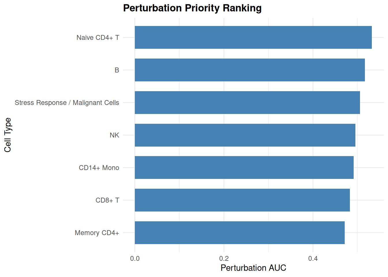
has_perturbation_priority() is worth calling first in any script that reads the record: it returns FALSE rather than erroring on an object where Augur never ran, which keeps a downstream report from failing on a partially analysed object.
Note that get_perturbation_priority() reads the analysis record ("augur"), not the typed state record. get_perturbation() is the CellOracle accessor and reads a different state type, so on an object where only Augur has run it returns NULL — the two names are easy to confuse and they do not overlap.
15.2 Rare Cell Detection
RunRareCellDetection(method = "density") labels small populations directly on the kNN graph of a reduction. It needs no Python, no annotation reference, and no condition labels — only BiocNeighbors (already a sclet dependency) and a PCA. The algorithm:
- Build the kNN graph on the chosen dimensions and compute each cell’s mutual connectivity
Q: the fraction of its k neighbours that list it as a neighbour too.Qis high where the graph is locally dense. - Seed on local maxima — a cell becomes a seed when its
Qexceeds the medianQof its own neighbours and clearsq_threshold. Adjacent seeds are merged through their mutual kNN links before anything propagates, because two adjacent dense cells belong to one density peak. - Propagate labels outward for five iterations, then dissolve any group smaller than
min_cluster_sizeinto its densest neighbouring group. - Flag every group with at most
rare_thresholdcells as rare.
Both the seeding rule and the dissolution step are the results of a measured failure, and the chapter should say so plainly. The first version of this seeding rule treated every cell above q_threshold as its own seed, and on PBMC 3k that produced 2419 “populations” for 2700 cells, 75% of them one cell. A one-cell population is where a cell happened to sit, not a population. The current rule — local maximum, merge adjacent seeds, dissolve what remains below min_cluster_size — is what makes the label column interpretable.
The first run is on the shared pbmc object, because that is the object every
chapter uses:
library(sclet)

# PCA already exists on pbmc from the core workflow.
rare_demo <- RunRareCellDetection(
    pbmc,
    method = "density",
    reduction = "PCA",
    dims = 1:10,
    k = 20,
    q_threshold = 0.25,
    rare_threshold = 10,
    name = "density_demo"
)

rare_info <- get_rare_cells(rare_demo)
c(n_clusters = rare_info$n_clusters,
  n_rare_clusters = rare_info$n_rare_clusters)
## n_clusters n_rare_clusters
## 4 0That run is a negative result, and it is a useful one: the PBMC 3k embedding
is a small number of broad blobs, so the density rule consolidates everything
and n_rare_clusters comes back 0. Nothing is wrong with the function — it is
reporting that the embedding has no small isolated peak. On a real dataset this
is the answer that tells you not to spend time on a follow-up.
To see the positive case, and to test the AI layer’s evidence grading, the chapter builds a small object with a population the clustering does separate. The fixture is 409 cells, three hundred genes, and a nine-cell block with twenty of its own up-regulated genes — small enough to render fast, structured enough that “rare population” means something:
set.seed(7)
n_genes <- 300
n_main <- 400
n_rare <- 9
rare_columns <- n_main + seq_len(n_rare)

fixture_counts <- matrix(
    rpois(n_genes * (n_main + n_rare), lambda = 3),
    nrow = n_genes,
    dimnames = list(paste0("gene_", seq_len(n_genes)),
        paste0("cell_", seq_len(n_main + n_rare))))
# The rare block is marked by genes the rest of the object does not express.
fixture_counts[seq_len(20), rare_columns] <- fixture_counts[seq_len(20), rare_columns] + 120

fixture <- SingleCellExperiment(list(counts = fixture_counts))
fixture <- NormalizeData(fixture)
fixture <- FindVariableFeatures(fixture, nfeatures = 150)
fixture <- RunPCA(fixture, ncomponents = 10)
fixture <- FindNeighbors(fixture, dims = 1:10)
fixture <- FindClusters(fixture, resolution = 0.5)

# The clustering already separates the small block.
table(SingleCellExperiment::colLabels(fixture))
##
## 1 2
## 400 9# k = 10 rather than the default 20: with k = 20 the 9-cell block's neighbours
# reach into the main blob and the group is dissolved. This is a property of
# small populations in general, not of the fixture -- k has to be small enough
# that a rare cell's neighbourhood stays inside the rare population.
fixture <- RunRareCellDetection(
fixture,
method = "density",
reduction = "PCA",
dims = 1:10,
k = 10,
rare_threshold = 10,
min_cluster_size = 2L,
name = "rareq"
)
fixture_counts_by_group <- table(fixture$rare_cluster)
fixture_counts_by_group##
## 1 2
## 400 9fixture_info <- get_rare_cells(fixture)
c(n_clusters = fixture_info$n_clusters,
n_rare_clusters = fixture_info$n_rare_clusters)## n_clusters n_rare_clusters
## 2 1The label column and the recorded counts agree: two groups, one of them the
nine-cell population, which rare_threshold = 10 flags as rare.
15.3 The Workflow Shell
RunStatePriorityWorkflow() runs either or both analyses and records them as one mainline record pointing at the component ids:
pbmc <- RunStatePriorityWorkflow(
    pbmc,
    condition_col = "condition",
    group_col = "colLabels",
    run_perturbation_priority = TRUE,
    run_rare_cell_detection = TRUE,
    name = "state_priority_main"
)
The shell refuses an empty request (needs at least one prioritization task enabled) rather than writing a workflow record that describes nothing. Note one asymmetry that is easy to trip over: the shell passes its own name-derived ids to the components (<name>_priority, <name>_rare) and forwards ... to those components. The rare-cell component is called with its defaults only, so reduction, dims and k for rare detection are not configurable through this shell — call RunRareCellDetection() directly when you need to change them.
15.4 The AI Layer: run_rare_cell_detection
The AI action layer exposes run_rare_cell_detection, which wraps RunRareCellDetection() and then writes one evidence node per small population. The action’s prerequisite is narrow and worth knowing: it needs the named reduction to exist (either on the object or as a planned reduction earlier in the same plan) and BiocNeighbors to be installed. It does not require condition labels — rare cell detection is not a condition analysis.
15.4.1 The ordering rule that costs a run to learn
This is the single most important practical fact about the action, and it is in AGENTS.md because it was measured on real billed runs:
run_de_testmust come beforerun_rare_cell_detectionin the plan.
The reason is in how evidence is graded. Each rare population’s evidence node is graded by n_independent_signals — the number of independent signal classes informative for that population at the moment the action runs. Four classes are considered: QC metrics, doublet calls, an attributable marker test, and sample replication. Cluster size alone is never a signal.
If the marker test has not run yet, the marker class is unavailable, and on an
object with no QC columns, no scDblFinder calls and no sample column either,
zero signal classes are available. The action then records nothing at all
and stamps a no_evidence_recorded note on the returned object. A plan can still
complete every step, the object still gains a rare_cluster column, and the
ledger holds no evidence — the “message and artifact disagree” shape of failure
that a plan validator cannot see, because ordering markers after rare detection
is not invalid, only useless.
The two runs below are the same fixture, same parameters, same population. The only difference is whether the marker test ran first:
registry <- AIDefaultExecutionRegistry(fixture, include = "all")

# --- Ordering A: rare detection on an object with no marker test. ---
rare_first <- registry$run_rare_cell_detection$handler(fixture,
    list(reduction = "PCA", dims = 1:10, k = 10, rare_threshold = 10,
        min_cluster_size = 2L, name = "rareq_A"))

# --- Ordering B: marker test first, then rare detection. ---
de_first <- RunDEtest(fixture, name = "findallmarkers")
de_first <- registry$run_rare_cell_detection$handler(de_first,
    list(reduction = "PCA", dims = 1:10, k = 10, rare_threshold = 10,
        min_cluster_size = 2L, name = "rareq_B"))
# Evidence nodes recorded under each ordering.
c(rare_first = length(sclet:::sclet_ai_evidence_get_all(rare_first)),
de_first = length(sclet:::sclet_ai_evidence_get_all(de_first)))## rare_first de_first
## 0 1Ordering A records nothing for the nine-cell group. Ordering B records one node, and its fields explain why the grade is what it is:
node <- sclet:::sclet_ai_evidence_get_all(de_first)[[1]]

unlist(node$values)[c("population_label", "population_size",
    "n_independent_signals", "marker_available",
    "sample_replication_available", "low_confidence")]
## population_label population_size
## "group_2" "9"
## n_independent_signals marker_available
## "1" "TRUE"
## sample_replication_available low_confidence
## "FALSE" "TRUE"## [1] "associated"One signal class is available — the marker test — so the claim is levelled
"associated" and the node is marked low_confidence = TRUE. Adding sample
replication or doublet calls would raise it to "consistent_with". The same
grading is available directly, without going through the action, which is the
call to make when you want to know before relying on a rare population how
much support it would have:
# Marker test first: an all-cluster marker run records markers per cluster, so
# each population can then be credited individually.
signals <- summarize_small_cluster_evidence(de_first, cluster = "rare_cluster",
    size_threshold = 10)
unlist(signals$independent_signals$marker)[c("available",
    "n_significant_up_genes")]
## available n_significant_up_genes
## 1 20## [1] 115.4.2 Why the whole thing is not executed through a plan
Everything above calls the registered handler directly. The full path —
AIPlanAnalysis() proposing a plan, ValidateAIPlan() approving it,
ExecuteAIPlan() running it — is a billed model call, so it runs only on a
machine with a provider configured (SCLET_BOOKDOWN_EVAL_AI=1). The handler is
the layer that writes the evidence, so calling it directly tests the same
ordering rule without a model in the middle.
plan <- AIPlanAnalysis(fixture,
    goal = "find rare populations and support them with marker evidence")

# What the planner proposed, in order. This is the part that varies.
vapply(plan$actions, function(step) step$action, character(1))
## [1] "run_de_test" "run_rare_cell_detection"# Three arguments are easy to get wrong here and none of them fails loudly:
# validation takes the plan FIRST, the token lives on the validation object,
# and `dry_run` defaults to TRUE -- omit it and the "execution" is a preview
# that reports `status = "dry_run"` with no evidence, which reads exactly like
# a plan that ran and found nothing.
validation <- ValidateAIPlan(plan, object = fixture, registry = registry)
if (isTRUE(validation$valid)) {
out <- ExecuteAIPlan(fixture, plan, registry,
validation = validation,
dry_run = FALSE,
confirmation = validation$confirmation_token)
evidence <- sclet:::sclet_ai_evidence_get_all(out$object)
c(status = out$status,
steps = length(out$results),
evidence_nodes = length(evidence))
} else {
# Refused before anything ran. This is the common outcome on this object,
# and the reason is the ordering rule above.
validation$errors
}## status steps evidence_nodes
## "completed" "2" "1"Three outcomes are all reachable here, and telling them apart is the skill this section is teaching:
- refused (
validation$validisFALSE, nothing runs): the plan is illegal for this object. The most likely reason onfixtureis ordering — it has already been throughRunRareCellDetection(), which leaves a single identity group (the rare labels live in their own column, not incolLabels), so a marker test placed after the detection has no second group to test against and fails its prerequisite. completed— every step ran. The evidence count says whether any of them left something citable;0is a real answer, not an error.failed— the plan was legal and a step still failed at run time. The steps before it may have recorded evidence, soevidence_nodescan be non-zero on a failed execution. Nothing is rolled back.
Which one you get changes between runs, because the planner is a language model and not a fixed recipe. So the chunk above reports the outcome it got instead of asserting the outcome it should have got — and that is the honest shape of AI-assisted analysis. The engine’s guarantee is narrow and worth stating precisely: the model proposes an order, the engine decides whether that order is legal, and neither of them promises that a legal order was a useful one.
15.5 What Fits Nearby
- Before this chapter: the core workflow for clustering, and reference mapping if you want
group_colto hold cell types rather than cluster codes. Augur’s ranking is only as interpretable as its groups. - Alongside this chapter: the Milo chapter answers the abundance question — did this neighbourhood change its cell count between conditions — where Augur answers the transcriptional question. A cell type can be highly responsive and unchanged in abundance, and the reverse, so the two tables are read together, not instead of each other.
- After this chapter: communication and spatial analysis can test whether the top-ranked states are also the ones whose signalling or location changed.
15.6 Current Recommendation
The recommendation has boundaries, because both methods are easy to over-read:
Use RunPerturbationPriority() when the question is “which of my annotated cell types respond transcriptionally to the perturbation”, you have at least two conditions with reasonable cell numbers per (cell type × condition) cell, and you are willing to install Augur from GitHub. Treat the AUC as an ordinal ranking with a null of 0.5, not as an effect size, and check that the top-ranked type is not simply the one with the most cells.
Do not use it when you have one sample per condition. Augur’s cross-validation operates within the pooled cells and does not model donor-level correlation, so a per-donor batch effect can be read as responsiveness. Milo’s mixed model (the Milo chapter) is the right tool for a sample-level design.
Use RunRareCellDetection(method = "density") when you suspect a small population was averaged into a larger cluster, and you want a cheap, deterministic, annotation-free labelling of candidate small populations on the embedding. It is suitable as a screening step: it tells you where to look.
Do not use it as evidence that a population is real. The label column is a density artefact detector, not a biological claim. A small population needs independent support — markers, doublet scores, QC behaviour, and replication across samples — which is exactly what the AI layer’s evidence grading encodes, and exactly why run_de_test has to run first. On the PBMC demo object the run consolidates everything and reports n_rare_clusters = 0: that is the method working.
When you want both, call RunStatePriorityWorkflow() with both flags for the convenience of one record, but call RunRareCellDetection() directly if you need to change reduction, dims, k, or min_cluster_size — the shell does not forward those.
15.7 What Is Not Here Yet
- No sample-level recombination for Augur.
RunPerturbationPriority()passes the pooled expression matrix toAugur::calculate_auc(). There is no per-donor cross-validation and no random effect, so a design with one sample per condition is not supported — use Milo. - No scCODA, no composition model of any kind.
sclethas no Bayesian compositional analysis for condition effects on cluster proportions. Milo covers neighbourhood abundance; scCODA-style compositional modelling of the cluster table does not exist here. - No CellOracle-level in-silico perturbation here. There is
RunInSilicoPerturbation()in the spatial mainline, which is a different thing: a GRN-based simulation. It is not connected to the priority ranking, and nothing lets you take “cell type 3 is the most responsive” and simulate a knockout in it in one call. - No second prioritization backend.
RunStatePriorityWorkflow()dispatches only Augur. The documentation of the shell says other prioritization modules “will be added as backends mature”; none is wired today, so a state-priority record’s only possible component isperturbation_priorityand/orrare_cells. - No rare-cell-evidence action other than the density method.
RunRareCellDetection()acceptsmethod = c("density")only. There is no UMAP-density variant, no label-propagation-from-markers variant, and no supervised rare-cell classifier. - The rare-cell evidence is not a p-value. Nothing here computes significance for a rare population. The evidence nodes record how many independent signal classes support the population and at what claim level, which is a calibration of confidence, not a test.