3 Cases
3.1 PBMC example
3.1.1 Marker gene heatmap
library(yulab.utils)
pload(dplyr)
pload(ggplot2)
pload(ggfun)
pload(ggtree)
pload(aplot)
pload(Seurat)


# celltype <- c("Naive CD4 T", "B", "NK")
# id <- pbmc@active.ident
# md = data.frame(cell=names(id), group=id)
# md <- md[md$group %in% celltype, ]
# md$group <- as.character(md$group)
# md <- lapply(split(md, md$group), function(x) x[1:30,]) |> rbindlist()
#
# pbmc <- pbmc[, md$cell]

pbmc <- readRDS("data/pbmc-subset.rds")

m <- FindAllMarkers(pbmc, only.pos=TRUE)

top10 <- m %>%
    group_by(cluster) %>%
    dplyr::filter(avg_log2FC > 2) %>%
    slice_head(n = 10)

pbmc <- ScaleData(pbmc, features = rownames(pbmc))
x  <- pbmc[['RNA']]$scale.data[top10$gene,]

y <- mat2df(x) -> y
y$gene <- rownames(x)[y$row]
y$cell <- colnames(x)[y$col]

p <- ggplot(y, aes(cell, gene, fill = value)) +
    geom_tile()+ scale_fill_viridis_c(name = "Gene Expression") +
    theme_noxaxis() +
    scale_y_discrete(position = "right") +
    xlab(NULL) +
    ylab(NULL)

gene_cls <- hclust(dist((x)))
cell_cls <- hclust(dist(t((x))))
gene_tree <- ggtree(gene_cls, branch.length = 'none')
cell_tree = ggtree(cell_cls, branch.length = 'none') + layout_dendrogram()


id <- pbmc@active.ident
md = data.frame(cell=names(id), group=id)
p_cell_type <- ggplot(md, aes(cell, y=1, fill = group)) +
    geom_tile() +
    scale_fill_brewer(palette="Set1", name = 'Cell Type') +
    theme_nothing()

g <- p |> insert_left(gene_tree, width = .2) |>
    insert_top(p_cell_type, height = .02) |>
    insert_top(cell_tree, height = .1)

g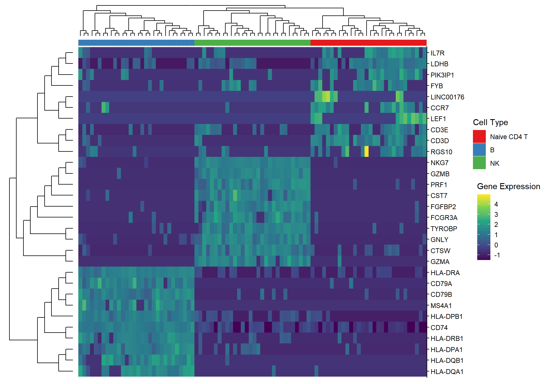
3.1.2 Degree of genes in the PPI network
pload(igraph)
pload(clusterProfiler)

ppi <- getPPI(top10$gene, output='igraph', taxID='9606')
deg <- stack(degree(ppi, v = V(ppi))) |> setNames(c("degree", "gene"))

p_ppi <- ggplot(deg, aes(1, gene, fill=degree, size=degree)) + geom_point(shape=21) +
    scale_fill_gradientn(colors = hcl.colors(20, "RdYlGn")) + theme_nothing()
3.1.3 Genes in pathways
pload(tidytree)
pload(msigdbr)

node <- c(35, 34, 32)
genes <- lapply(node, function(n) offspring(gene_tree, n, tiponly=T)$label) |>
    setNames(c("CD4", "NK", "B"))

pload(clusterProfiler)
gene_set <- msigdbr(species="human", category="C2")
names(gene_set)
## [1] "gene_symbol" "ncbi_gene"
## [3] "ensembl_gene" "db_gene_symbol"
## [5] "db_ncbi_gene" "db_ensembl_gene"
## [7] "source_gene" "gs_id"
## [9] "gs_name" "gs_collection"
## [11] "gs_subcollection" "gs_collection_name"
## [13] "gs_description" "gs_source_species"
## [15] "gs_pmid" "gs_geoid"
## [17] "gs_exact_source" "gs_url"
## [19] "db_version" "db_target_species"
## [21] "entrez_gene" "gs_cat"
## [23] "gs_subcat"cc <- compareCluster(genes, enricher, TERM2GENE=gene_set[, c("gs_name", "gene_symbol")])
res <- cc@compareClusterResult |>
group_by(Cluster) |>
slice_head(n = 5) |>
as.data.frame()
gene2path <- lapply(res$geneID, function(x) unlist(strsplit(x, split="/"))) |>
setNames(res$Description) |>
stack() |>
setNames(c("gene", "pathway"))
pcp <- ggplot(gene2path, aes(pathway, gene)) +
geom_point(size=5, shape=21, fill = "steelblue") +
theme_minimal() +
theme_noyaxis() +
theme(axis.text.x = element_text(angle=30, hjust=1)) +
xlab(NULL) +
ylab(NULL)
gg <- g |> insert_right(p_ppi, width=.05) |>
insert_right(pcp, width=.5)
gg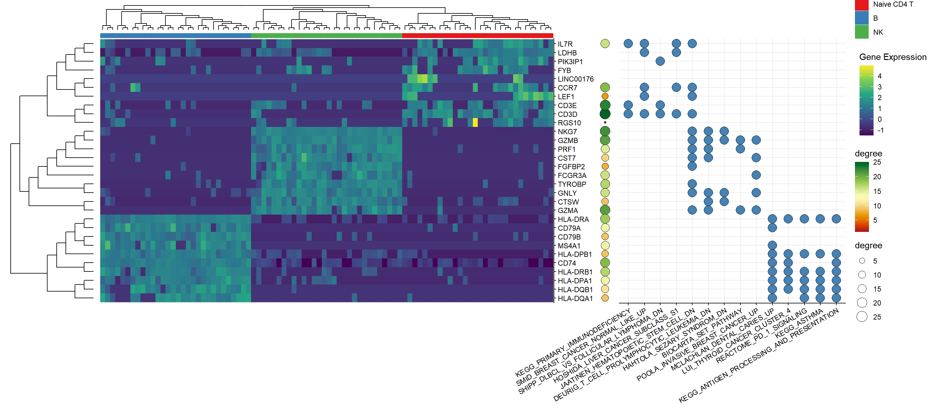
3.1.4 All in one
pp <- plot_list(cell_tree, p_cell_type, heights=c(1, .5))
pp <- plot_list(gene_tree, pp, widths=c(.3, 1))
pp <- plot_list(p, pp, p_ppi, pcp, widths=c(1, .8, .05, .6))
pp <- pp + patchwork::plot_annotation(tag_levels='a')

final_plot <- plot_list(pp, gg, ncol=1, tag_levels='A', heights=c(1, 1.2))
final_plot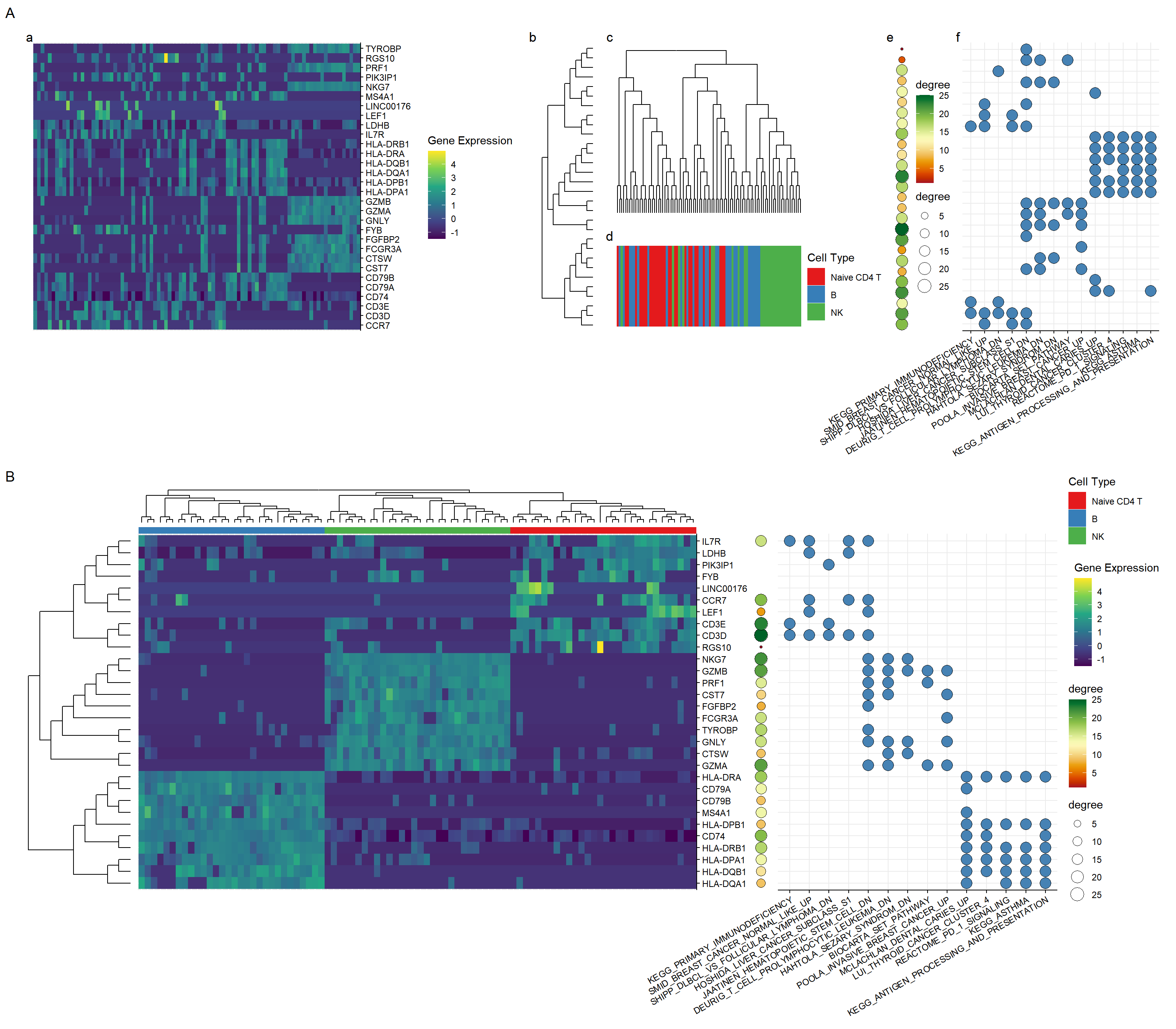
3.2 Oncoplot example
pload(aplotExtra)
pload(RTCGA.mRNA)
pload(RTCGA)

laml.maf <- system.file("extdata", "tcga_laml.maf.gz", package = "maftools")
laml.clin <- system.file('extdata', 'tcga_laml_annot.tsv', package = 'maftools')
laml <- maftools::read.maf(maf = laml.maf, clinicalData = laml.clin)
## -Reading
## -Validating
## -Silent variants: 475
## -Summarizing
## -Processing clinical data
## -Finished in 0.232s elapsed (0.280s cpu)onco <- oncoplot(maf = laml, genes = 20)
plot_tcga_expr <- function(mRNA, genes, name = "Gene Expression") {
d = expressionsTCGA(mRNA, extract.cols = genes)
dd = gather(d, gene, expression, -c(1,2))
ggplot(dd, aes(expression, gene, fill=stat(x))) +
ggridges::geom_density_ridges_gradient() +
scale_fill_viridis_c(option="C", name = name) +
theme_minimal() +
theme_noyaxis() +
xlab(NULL) +
ylab(NULL) +
theme(legend.position='bottom')
}
onco_genes <- aplotExtra:::get_oncoplot_genes(laml)
brca <- plot_tcga_expr(BRCA.mRNA, onco_genes, "Gene Expression in TCGA\nbreast cancer patients")
ov <- plot_tcga_expr(OV.mRNA, onco_genes, "Gene Expression in TCGA\novarian cancer patients")
op <- insert_right(onco, brca, width = .6) |>
insert_right(ov, width=.6)
op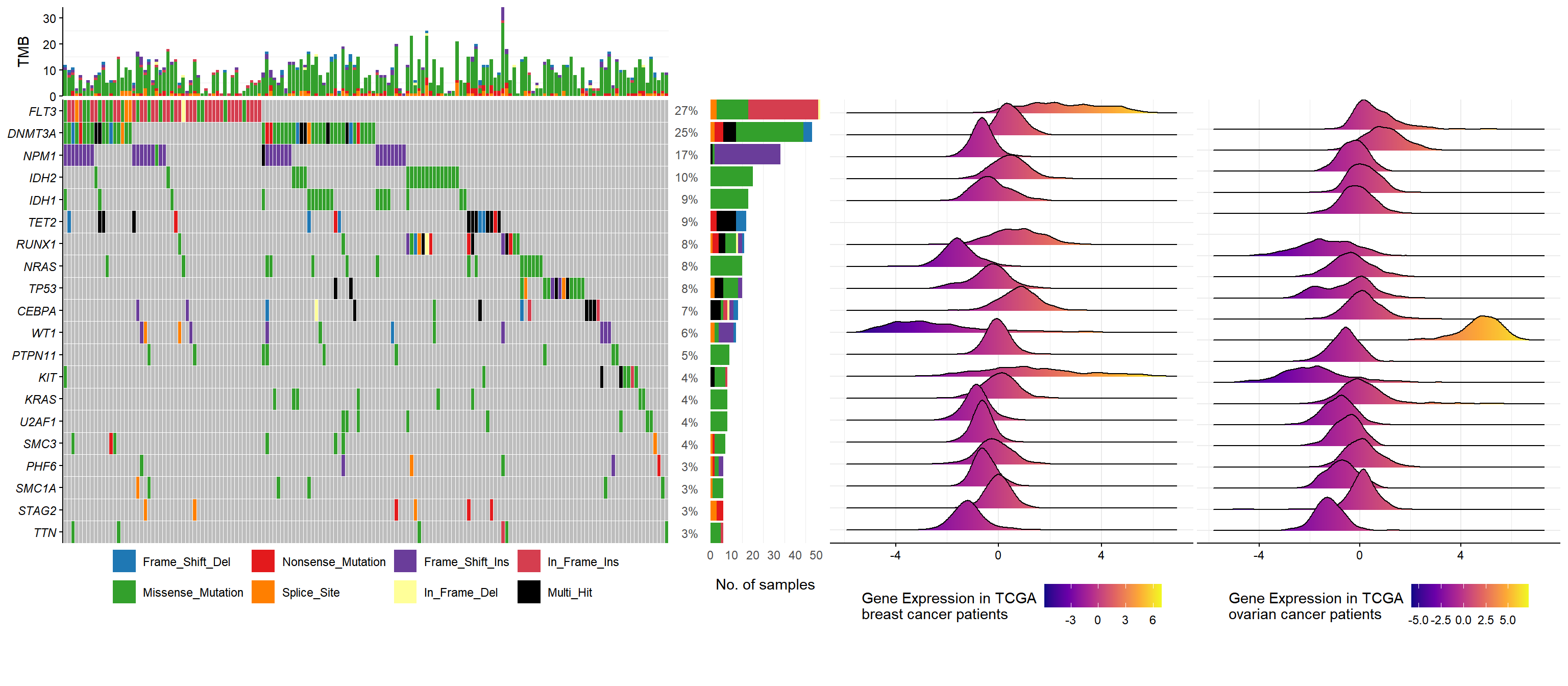
3.3 funky heatmap
library(aplotExtra)
library(tidyverse)
data("mtcars")


d <- yulab.utils::scale_range(mtcars) |>
    rownames_to_column("id") |>
    arrange(desc(mpg))


g1 <- funky_text(d)
g2 <- funky_bar(d, 2) + scale_fill_gradient(low = "#CC4C02", high = "#FFFFE5")
g3 <- funky_bar(d, 3) + scale_fill_gradient(low = "steelblue", high = "firebrick")
g4 <- funky_point(d, 4:7) + scale_fill_gradient(low = "#CC4C02", high = "#FFFFE5")
g5 <- funky_point(d, 8:12) + scale_fill_gradient(low = "#08519C", high = "#F7FBFF")


#funky_heatmap(data=mtcars)
fp <- funky_heatmap(g1, g2, g4, g5, options=theme_stamp())
fp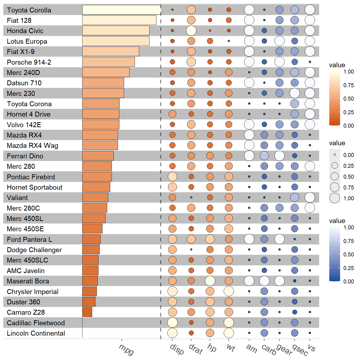
3.4 Genomics track example
3.4.1 Setup packages and parameteres
pload(ChIPseeker)
pload(TxDb.Hsapiens.UCSC.hg19.knownGene)
pload(org.Hs.eg.db)
pload(IRanges)
pload(GenomicFeatures)
pload(gggenes)
pload(HiContacts)
pload(cowplot)

# This analysis uses processed genomic data from:
# 1. Hi-C data: GM12878 (GSM1551550) and K562 (GSM1551618)
# 2. ChIP-seq data for histone modifications:
#    - H3K27ac (GM12878: GSM733771, K562: GSM733656)
#    - H3K4me1 (GM12878: GSM733772, K562: GSM733692)
#    - H3K4me3 (GM12878: GSM733708, K562: GSM733680)
#    - H3K36me3 (GM12878: GSM733679, K562: GSM733714)
#    Controls: GM12878 (GSM733742), K562 (GSM733780)

# Analysis parameters:
# - MACS2 peak calling: default parameters except:
#   * genome size: -g 2.7e9 (human)
# - MACS2 bdgdiff: default parameters except:
#   * d1: 6284864 (GM12878 sequencing depth) and d2: 18559220 (K562 sequencing depth)

# Load processed genomic data
epigenetics_data <- readRDS("./data/epigenetics_data.rds")

# Global parameters and themes
plot_params <- list(
    scale = "log10",
    limits = c(0, 1.7),
    chr = "chr6",
    x_min = 43600000,
    x_max = 44100000,
    highlight_regions = list(
        region1 = c(43738000, 43754500),
        region2 = c(43900000, 44000000),
        region3 = c(44060000, 44100000)
    ),
    peak_color = c("peak_in_K562" = "#E05B5B", "peak_in_GM12878" = "#519CBA")
)

common_theme <- theme_minimal() +
    theme(
        axis.title.x = element_blank(),
        panel.grid.minor = element_blank(),
        axis.line = element_line(colour = "black"),
        panel.border = element_blank(),
        plot.title = element_text(hjust = 0.5)
    )

txdb <- TxDb.Hsapiens.UCSC.hg19.knownGene

# Function to add highlight rectangles
addHighlights <- function(p, ymax, alpha=0.2) {
    p +
    annotate("rect",
             xmin=plot_params$highlight_regions$region1[1],
             xmax=plot_params$highlight_regions$region1[2],
             ymin=0, ymax=ymax, fill="#c6c3c3", alpha=alpha) +
    annotate("rect",
             xmin=plot_params$highlight_regions$region2[1],
             xmax=plot_params$highlight_regions$region2[2],
             ymin=0, ymax=ymax, fill="#c6c3c3", alpha=alpha) +
    annotate("rect",
             xmin=plot_params$highlight_regions$region3[1],
             xmax=plot_params$highlight_regions$region3[2],
             ymin=0, ymax=ymax, fill="#c6c3c3", alpha=alpha)
}

# Generate gene plot
generateGenePlot <- function(txdb, chr, x_min, x_max, OrgDb, show_legend = FALSE) {
    # Get genes in the region
    win <- GRanges(seqnames = chr,
                   ranges = IRanges::IRanges(start = x_min, end = x_max))
    all_genes <- GenomicFeatures::genes(txdb)
    gene_df <- data.frame(subsetByOverlaps(x = all_genes, ranges = win, type = "any"))
    gene_df$gene_id <- factor(gene_df$gene_id, levels = unique(gene_df$gene_id))

    # Process gene data
    gene_df <- gene_df[,c("seqnames", "gene_id", "start", "end", "strand")]
    colnames(gene_df)[1] <- "chromosome"
    gene_df$forward <- ifelse(gene_df$strand=="+", TRUE, FALSE)

    # Convert gene IDs
    changeid <- bitr(geneID = gene_df$gene_id,
                     fromType = "ENTREZID", toType = "SYMBOL",
                     OrgDb = OrgDb)
    colnames(changeid)[1] <- c("gene_id")
    gene_df <- merge(gene_df, changeid, all.x = TRUE)
    gene_df <- gene_df[, c(2:ncol(gene_df))]
    colnames(gene_df)[ncol(gene_df)] <- "gene_symbol"

    gene_df$start <- pmax(gene_df$start, x_min)
    gene_df$end <- pmin(gene_df$end, x_max)

    p <- ggplot(gene_df, aes(xmin = start, xmax = end,
                  y = gene_symbol, forward=forward, fill = gene_symbol)) +
    geom_gene_arrow() +
    xlim(c(x_min, x_max)) +
    theme_genes() +
    scale_fill_brewer(palette = "Set3") +
    labs(fill = "gene symbol") +
    common_theme

    if (!show_legend) {
        p <- p + theme(legend.position = "none")
    }

    return(p)
}

# Generate HiC plot
generateHicPlot <- function(data, label, use_scores = NULL, show_legend = TRUE) {
    if (is.null(use_scores)) {
        p <- HiContacts::plotMatrix(data,
            maxDistance = plot_params$x_max - plot_params$x_min,
            caption = FALSE,
            scale = plot_params$scale,
            limits = plot_params$limits) +
            xlim(plot_params$x_min, plot_params$x_max) +
            labs(fill = 'hic score') +
            ylab(paste0(label, " hic")) +
            common_theme
    } else {
        p <- HiContacts::plotMatrix(data,
            maxDistance = plot_params$x_max - plot_params$x_min,
            use.scores = use_scores,
            caption = FALSE,
            cmap = HiContacts::bbrColors()) +
            xlim(plot_params$x_min, plot_params$x_max) +
            labs(fill = 'log2fc') +
            ylab(paste0(label, " ")) +
            common_theme
    }

    if (!show_legend) {
        p <- p + theme(legend.position = "none")
    }

    return(p)
}

# Generate coverage plot
generateCoveragePlot <- function(data, label, ymax, colors = NULL,
                                add_facet = FALSE, show_legend = TRUE) {
    p <- covplot(data,
        weightCol = "V5",
        chrs = plot_params$chr,
        xlim = c(plot_params$x_min, plot_params$x_max),
        ylab = label,
        title = "") +
        ylim(c(0, ymax)) +
        common_theme

    if (!is.null(colors)) {
        p <- p + scale_color_manual(values = colors) +
                 scale_fill_manual(values = colors)
    } else {
        p <- p + scale_fill_brewer(palette = "Set2") +
                 scale_color_brewer(palette = "Set2")
    }

    if (add_facet) {
        p <- p + facet_grid(.id ~ .) +
            theme(strip.text.y = element_blank())
    }

    if (!show_legend) {
        p <- p + theme(legend.position = "none")
    }

    return(p)
}
3.4.2 Visualization of comparative genomics data tracks
# Generate HiC comparision plot
combine_hic_p <- generateHicPlot(epigenetics_data[["div_hic"]],
                                "K562/GM12878 hic compare",
                                use_scores = "balanced.fc")

# Generate histone modification comparision plots
histone_plots <- list(
    H3K27ac = list(data = epigenetics_data[["H3K27ac_peak"]], ymax = 100),
    H3K36me3 = list(data = epigenetics_data[["H3K36me3_peak"]], ymax = 10),
    H3K4me1 = list(data = epigenetics_data[["H3K4me1_peak"]], ymax = 30),
    H3K4me3 = list(data = epigenetics_data[["H3K4me3_peak"]], ymax = 25)
) %>%
map2(names(.), function(x, name) {
    p <- generateCoveragePlot(x$data, name, x$ymax,
                             plot_params$peak_color, add_facet = FALSE)
    addHighlights(p, x$ymax)
})

# Generate gene track
gene_p <- generateGenePlot(txdb = txdb,
                   chr = plot_params$chr,
                   x_min = plot_params$x_min,
                   x_max = plot_params$x_max,
                   OrgDb = "org.Hs.eg.db")
gene_p_highlighted <- addHighlights(gene_p, ymax=9)

# Combine all plots using aplot
combined_p <- combine_hic_p %>%
    insert_bottom(histone_plots$H3K27ac, height = .2) %>%
    insert_bottom(histone_plots$H3K36me3, height = .2) %>%
    insert_bottom(histone_plots$H3K4me1, height = .2) %>%
    insert_bottom(histone_plots$H3K4me3, height = .2) %>%
    insert_bottom(gene_p_highlighted, height = .5)

combined_p
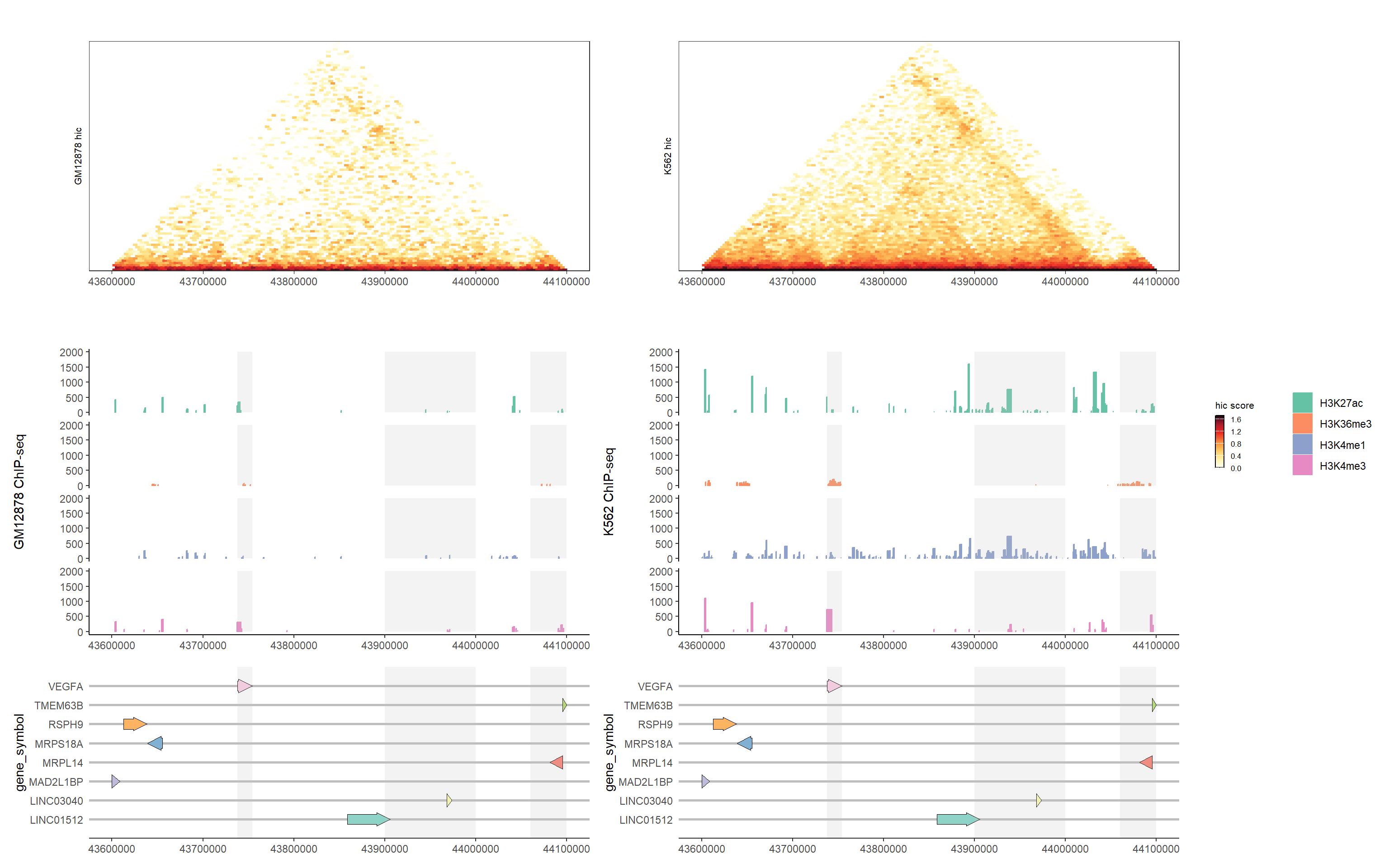
3.4.3 Visualization of different genomics data tracks
# Generate HiC plots
GM12878_hic_p <- generateHicPlot(epigenetics_data[["GM12878_hic"]],
                                "GM12878", show_legend = FALSE)
K562_hic_p <- generateHicPlot(epigenetics_data[["K562_hic"]],
                             "K562", show_legend = FALSE)

# Generate ChIP-seq coverage plots
GM12878_cov_p <- generateCoveragePlot(epigenetics_data[["GM12878_peak"]],
                                     "GM12878 ChIP-seq",
                                     2000,
                                     add_facet = TRUE,
                                     show_legend = FALSE)
GM12878_cov_p <- addHighlights(GM12878_cov_p, ymax = 2000)

K562_cov_p <- generateCoveragePlot(epigenetics_data[["K562_peak"]],
                                  "K562 ChIP-seq",
                                  2000,
                                  add_facet = TRUE,
                                  show_legend = FALSE)
K562_cov_p <- addHighlights(K562_cov_p, ymax = 2000)

# Combine plots using aplot
GM12878_p <- (GM12878_hic_p + theme(legend.position = 'none'))  %>%
             insert_bottom(GM12878_cov_p) %>%
             insert_bottom(gene_p_highlighted, height = .6)

K562_p <- (K562_hic_p + theme(legend.position = 'none')) %>%
             insert_bottom(K562_cov_p) %>%
             insert_bottom(gene_p_highlighted, height = .6)

# Add legends and create final view
split_p <- plot_list(
    gglist = list(GM12878_p, K562_p,
                 plot_grid(get_legend(generateHicPlot(epigenetics_data[["K562_hic"]], "K562")),
                          get_legend(generateCoveragePlot(epigenetics_data[["K562_peak"]],
                                                       "K562 ChIP-seq",
                                                       2000,
                                                       add_facet = TRUE)),
                          nrow = 1)),
    design = c("AAAAAABBBBBBCC")
)

split_p