1 Visualizing Seurat objects
library(Seurat)
dir = "data/filtered_gene_bc_matrices/hg19"

pbmc.data <- Read10X(data.dir = dir)
pbmc <- CreateSeuratObject(counts = pbmc.data, project = "pbmc3k",
                          min.cells=3, min.features=200)
pbmc
## An object of class Seurat
## 13714 features across 2700 samples within 1 assay
## Active assay: RNA (13714 features, 0 variable features)
## 1 layer present: countspbmc[["percent.mt"]] <- PercentageFeatureSet(pbmc, pattern = "^MT-")
pbmc <- subset(pbmc,
subset = nFeature_RNA > 200 & nFeature_RNA < 2500 & percent.mt < 5
)pbmc <- NormalizeData(pbmc, normalization.method = "LogNormalize",
scale.factor = 10000)
pbmc <- ScaleData(pbmc)pbmc <- FindVariableFeatures(pbmc, selection.method = "vst",
nfeatures = 2000)
pbmc <- RunPCA(pbmc, features = VariableFeatures(object = pbmc))
pbmc <- RunUMAP(pbmc, dims = 1:10)## Modularity Optimizer version 1.3.0 by Ludo Waltman and Nees Jan van Eck
##
## Number of nodes: 2638
## Number of edges: 95927
##
## Running Louvain algorithm...
## Maximum modularity in 10 random starts: 0.8728
## Number of communities: 9
## Elapsed time: 0 seconds## Assigning cell type identity to clusters
cluster.ids <- c("Naive CD4 T", "CD14+ Mono", "Memory CD4 T",
"B", "CD8 T", "FCGR3A+ Mono", "NK", "DC", "Platelet")
names(cluster.ids) <- levels(pbmc)
pbmc <- RenameIdents(pbmc, cluster.ids)1.1 Dimensional reduction plot
# DimPlot(pbmc, reduction = "umap",
#        label = TRUE, pt.size = 0.5)

library(ggplot2)
library(ggsc)

sc_dim(pbmc) + sc_dim_geom_label()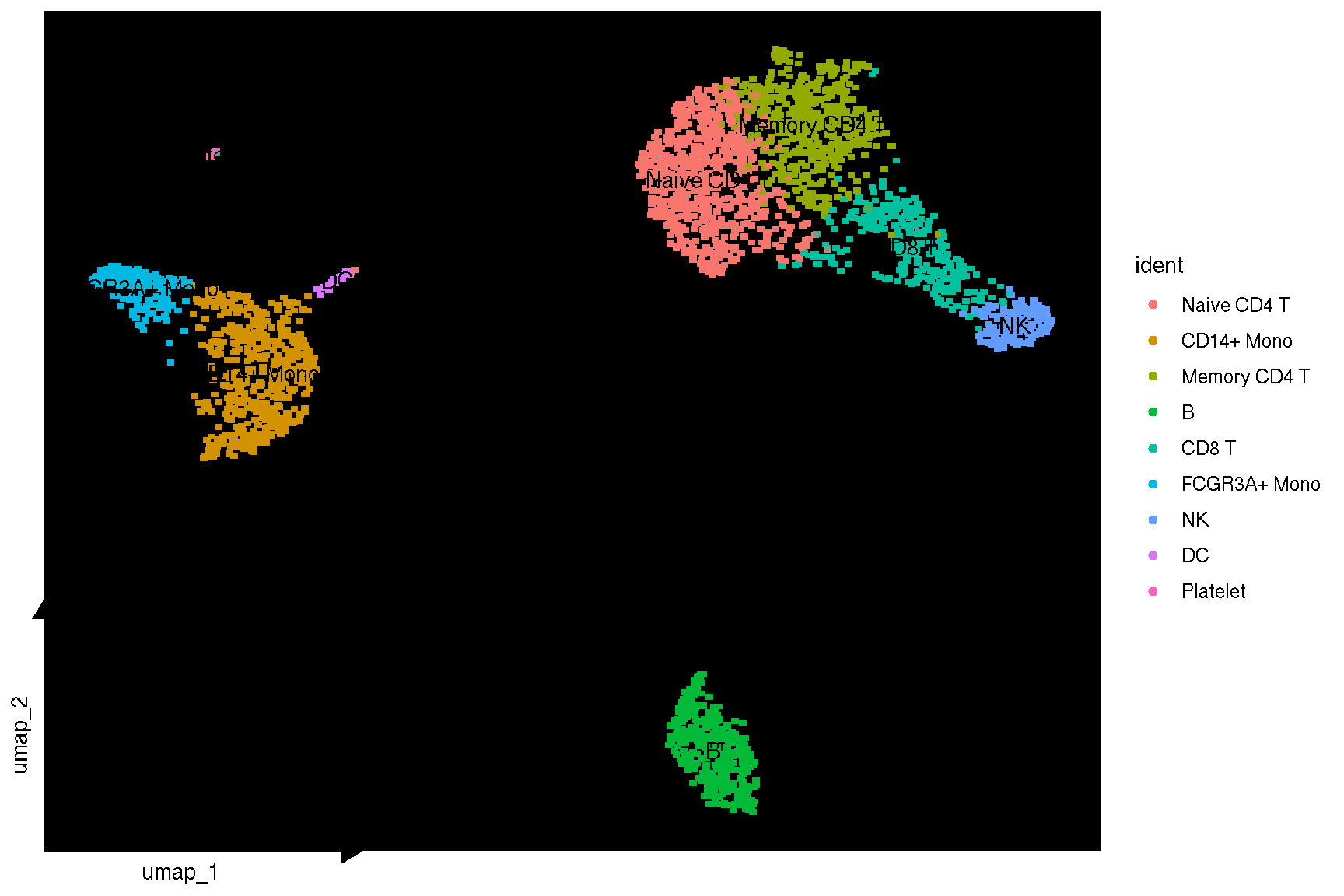
# using vector point layer when geom = geom_bgpoint
sc_dim(pbmc, geom = geom_bgpoint, pointsize=1) + sc_dim_geom_label()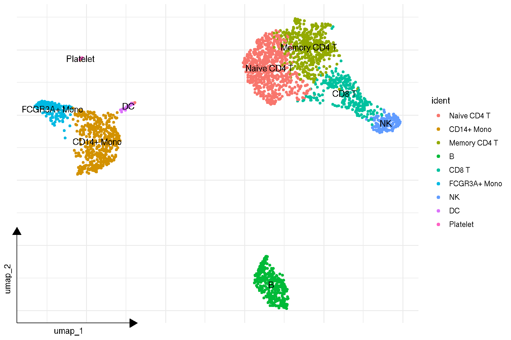
p <- sc_dim(pbmc) +
    sc_dim_geom_label(geom = shadowtext::geom_shadowtext,
            color='black', bg.color='white')
p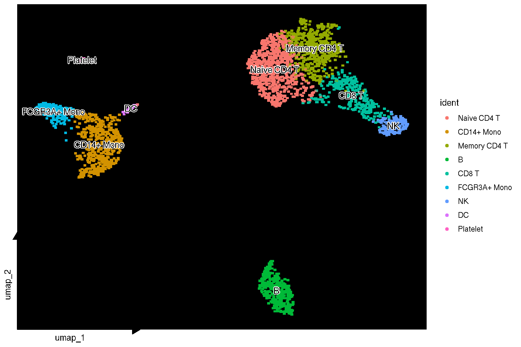
f <- sc_dim(pbmc, bg_colour = 'black') +
    sc_dim_geom_label(geom = shadowtext::geom_shadowtext,
    color = 'black', bg.color='white')
f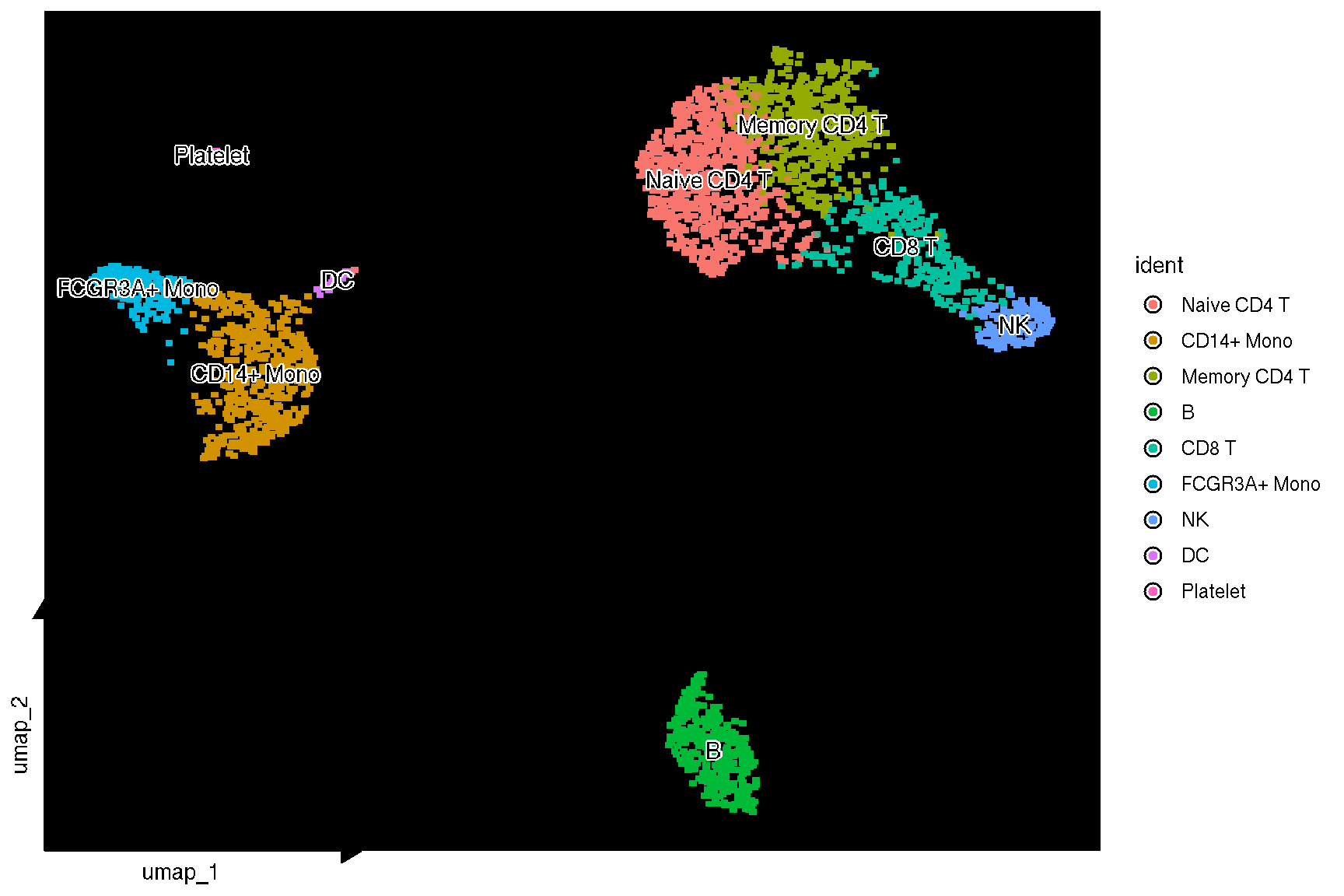
f2 <- sc_dim(pbmc,
             mapping = aes(bg_colour = ident),
             geom = geom_bgpoint,
             pointsize=1,
         gap_line_width=.2
      ) +
      sc_dim_geom_label(geom = shadowtext::geom_shadowtext,
      color = 'black', bg.color='white')
f2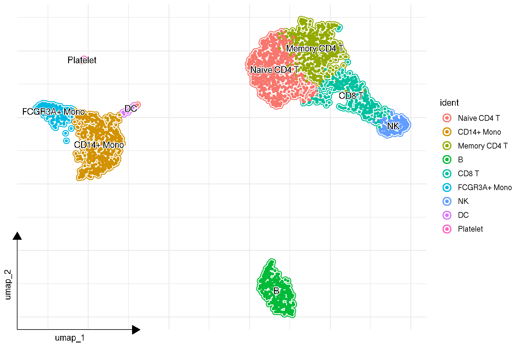
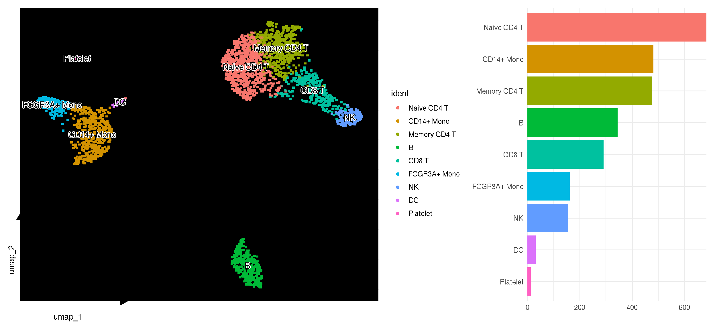
The number of cells in each clusters can be easily Visualized using sc_dim_count(). The colors of the bar plot is consistent with the dimensional reduction plot.
library(dplyr)

top20 <- pbmc.markers |>
    dplyr::group_by(cluster) |>
    dplyr::filter(avg_log2FC > 1) |>
    dplyr::slice_head(n = 20) |>
    dplyr::ungroup()

library(clusterProfiler)
library(enrichplot)

gg <- bitr(top20$gene, 'SYMBOL', 'ENTREZID', 'org.Hs.eg.db')
top20 <- merge(top20, gg, by.x='gene', by.y = 'SYMBOL')

kk <- compareCluster(ENTREZID~cluster, data = top20, fun=enrichKEGG)
g <- dotplot(kk, label_format=100) +
aes(x=sub("\n.*", "", Cluster)) +
xlab("Cell Clusters") +
ggtitle(NULL) +
theme(axis.text.x = element_text(angle=30, hjust=1))
p3 <- p2 + coord_cartesian() +
ggfun::theme_noxaxis() +
xlab(NULL)
insert_top(g, p3, height=.2)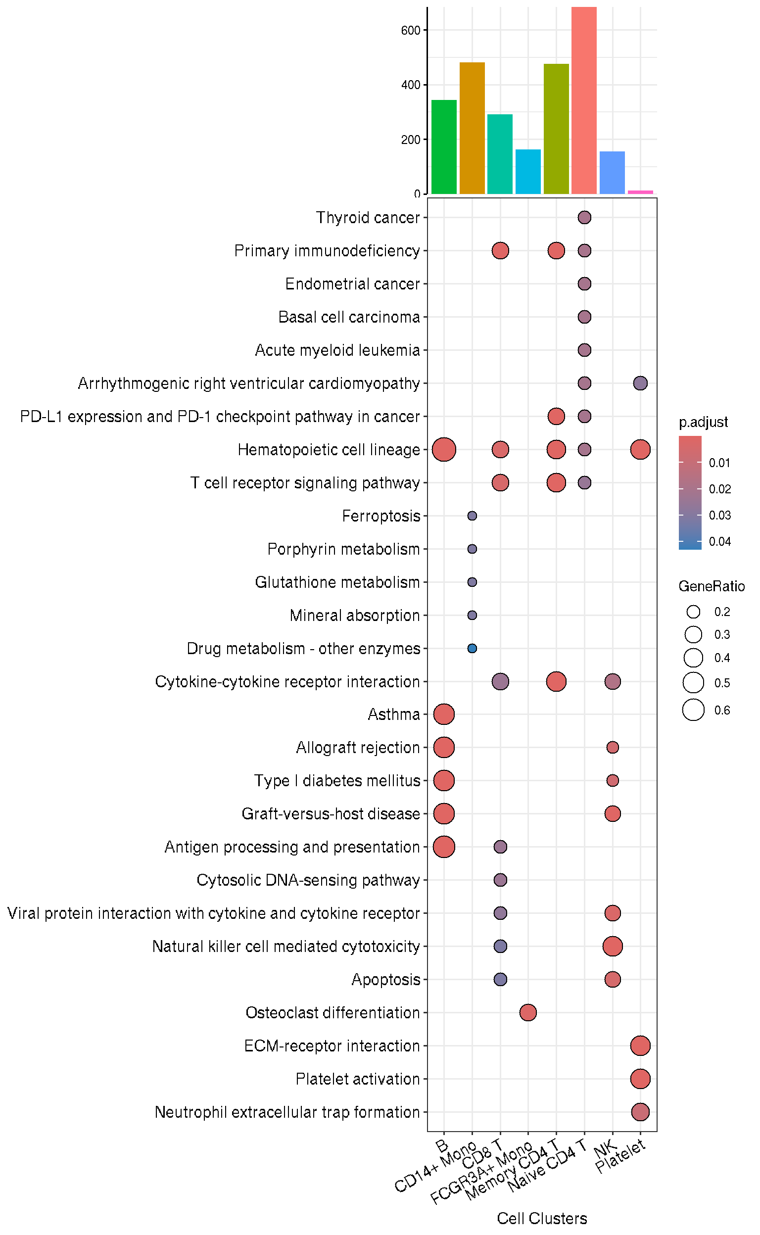
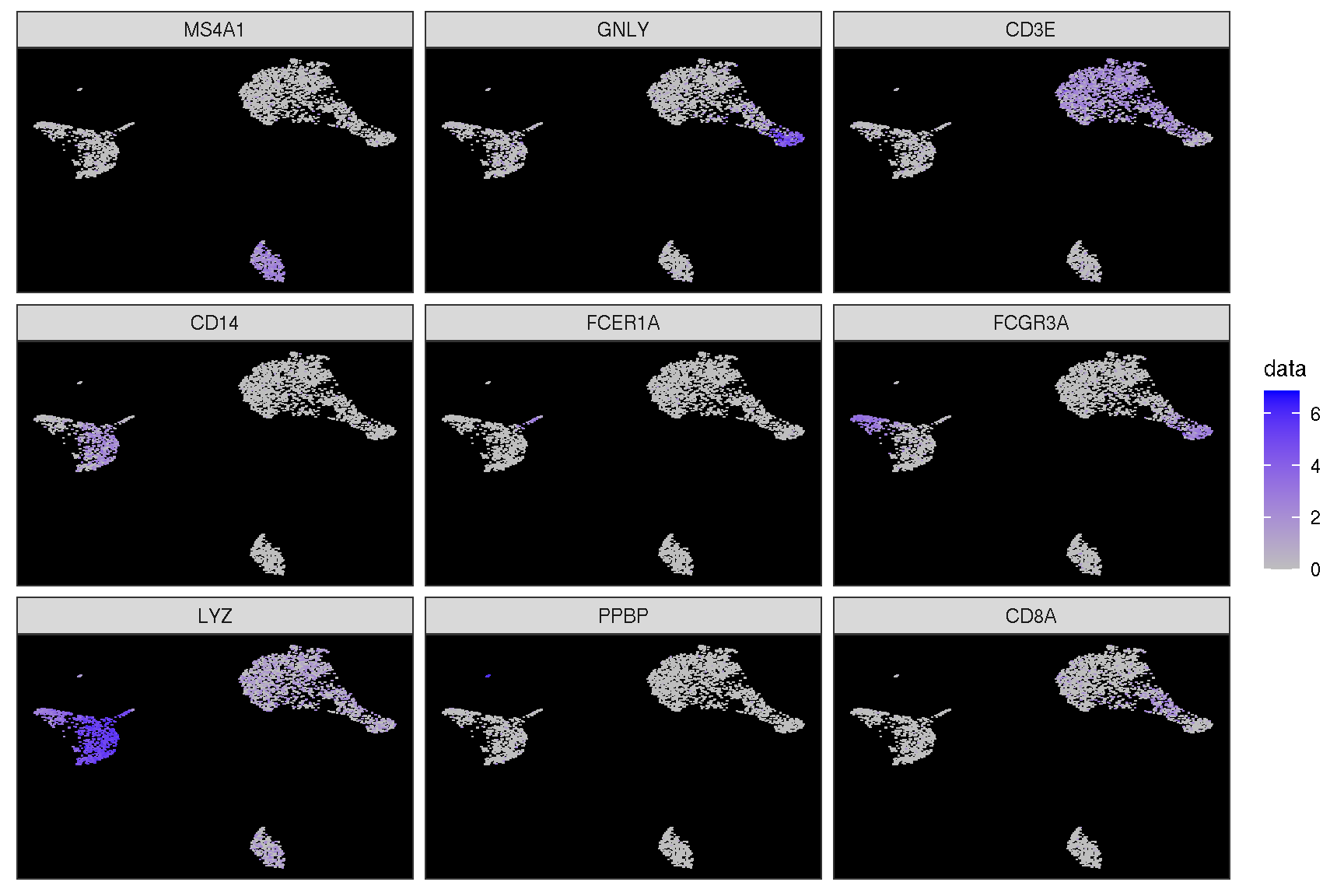
1.2 Visualize ‘features’ on a dimensional reduction plot
features = c("MS4A1", "GNLY", "CD3E",
            "CD14", "FCER1A", "FCGR3A",
            "LYZ", "PPBP", "CD8A")

# FeaturePlot(pbmc,'CD4')
sc_feature(pbmc, 'CD4')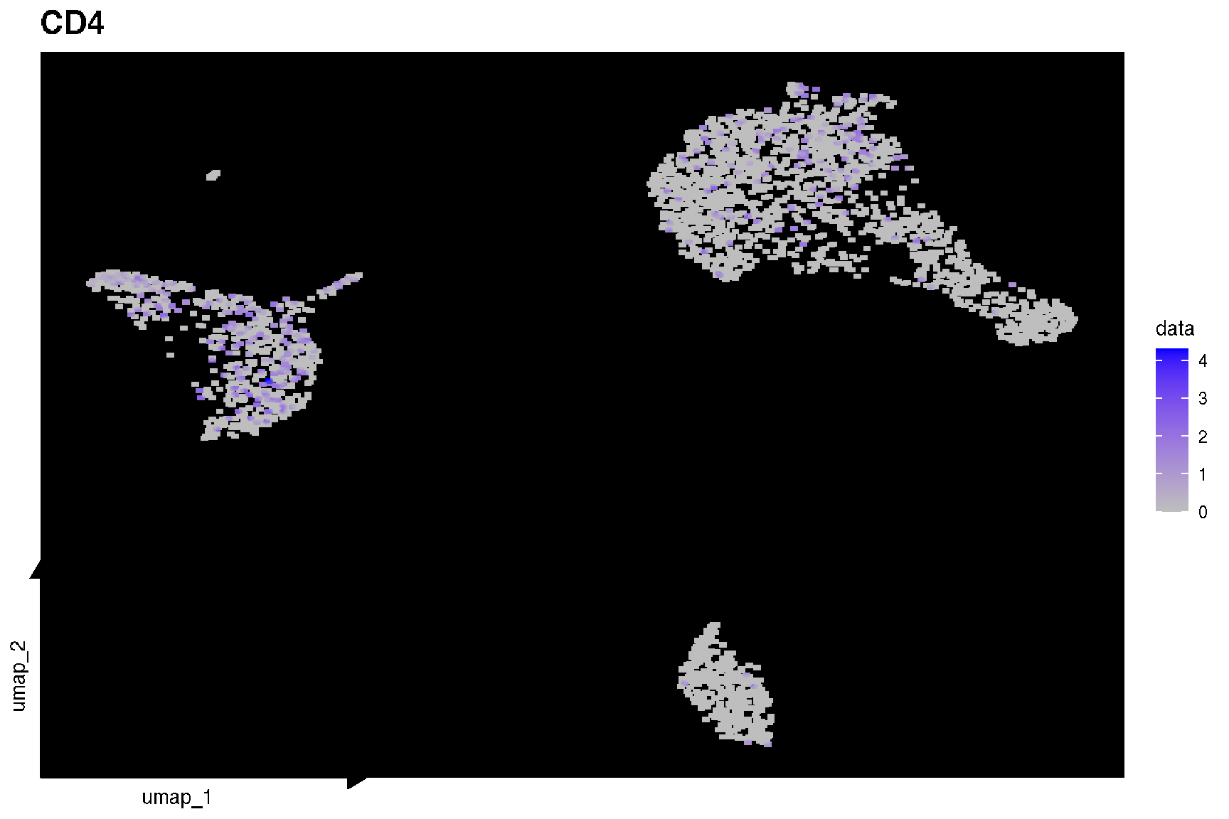
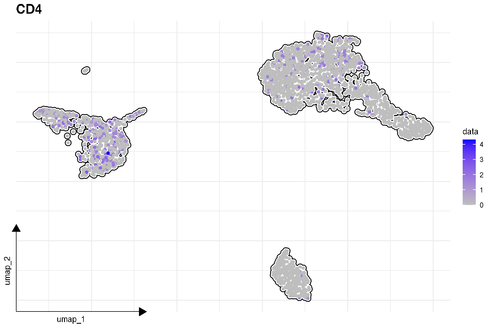
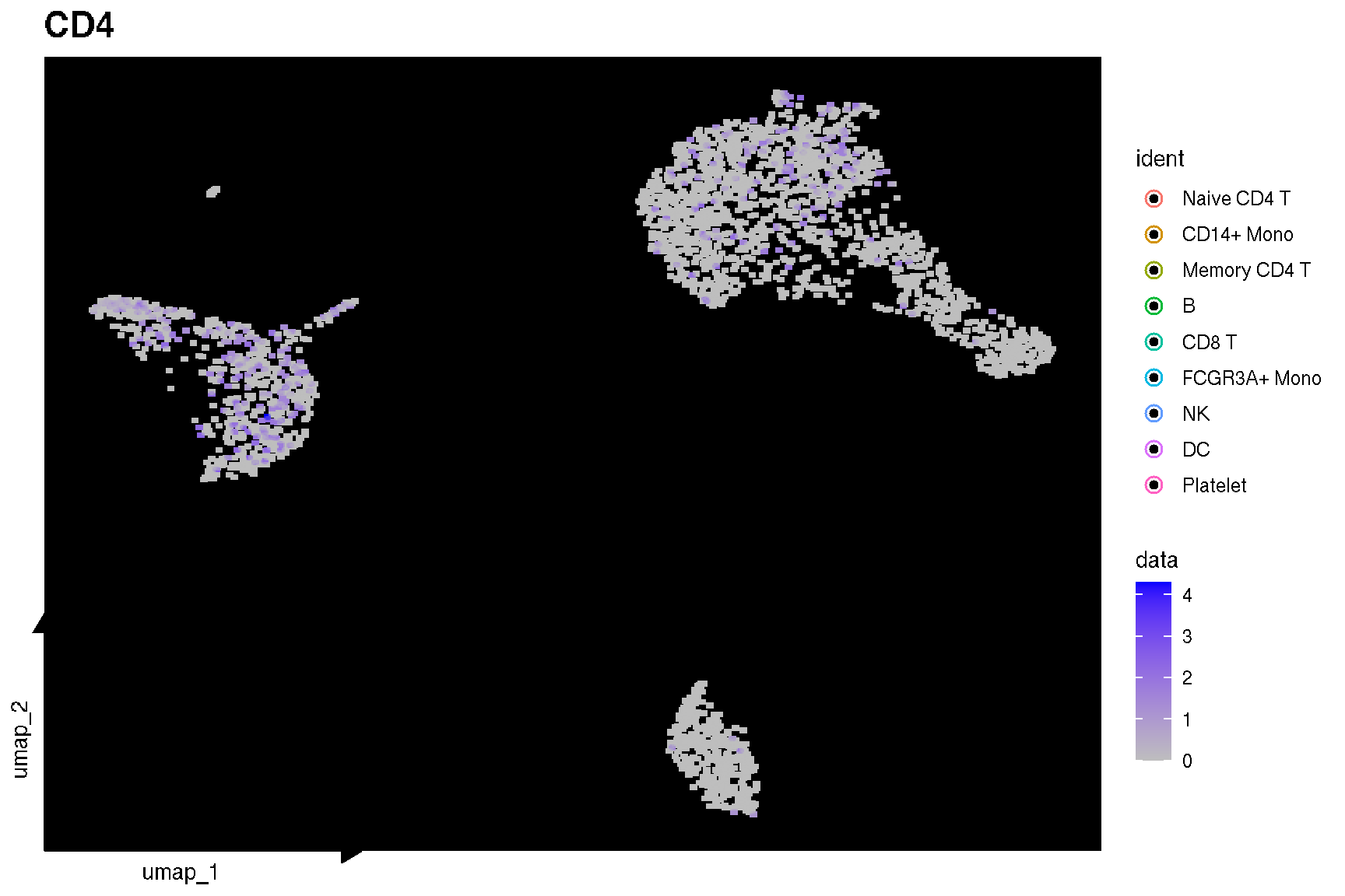
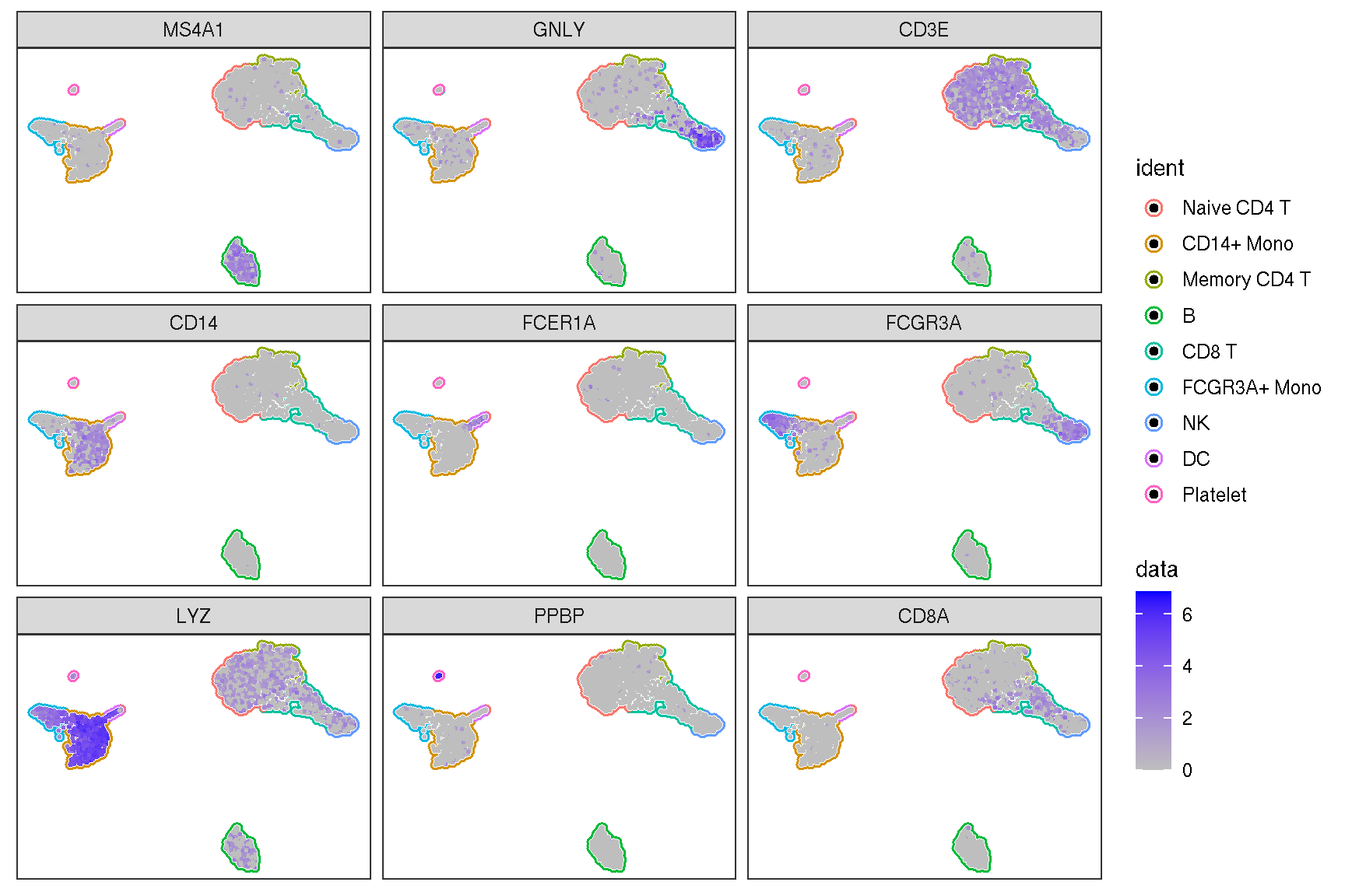
Here is the real ‘features’ on dimensional plot
sc_dim(pbmc, alpha=.3) +
    ggnewscale::new_scale_color() +
    sc_dim_geom_feature(pbmc, features, mapping=aes(color=features)) +
    scale_color_viridis_d()
sc_dim(pbmc, alpha=.3) +
    ggnewscale::new_scale_color() +
    sc_dim_geom_feature(pbmc, features, mapping=aes(color=features)) +
    scale_color_viridis_d()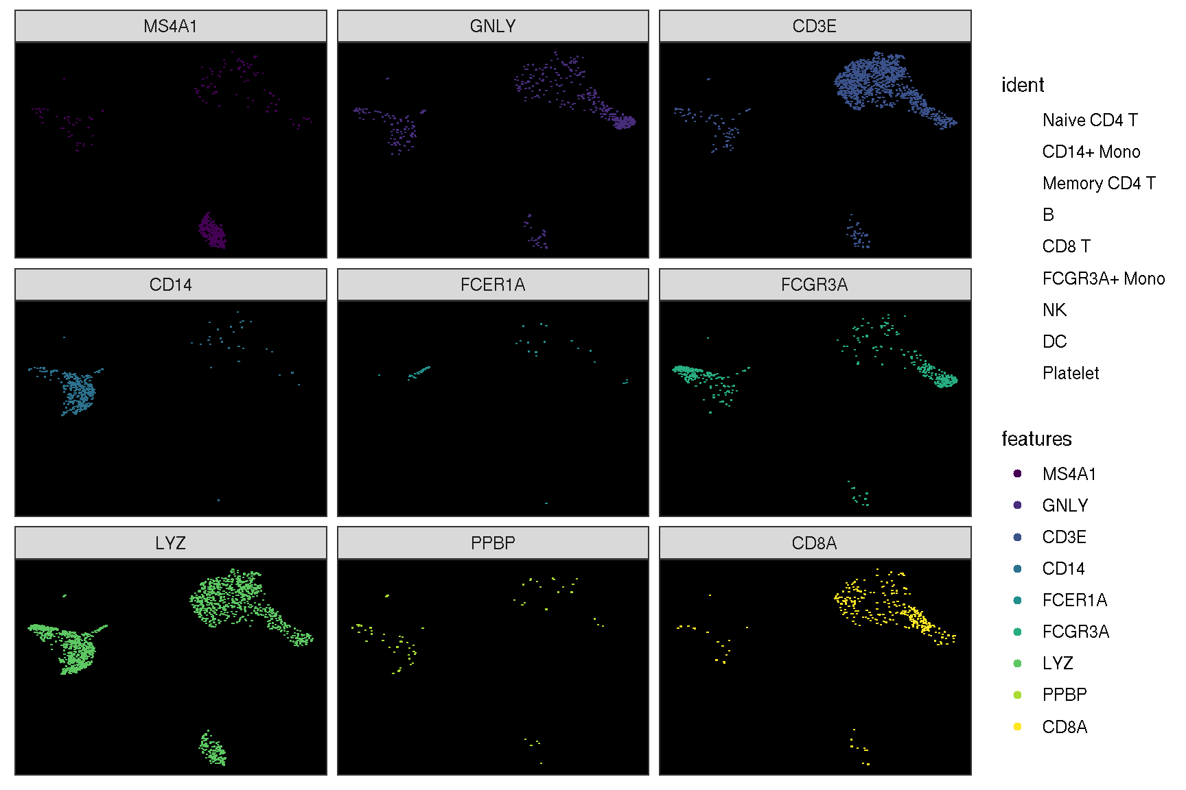
p1 <- sc_feature(pbmc, features='CD3E', density = FALSE) + scale_color_viridis_c()
p2 <- sc_feature(pbmc, features='CD3E', density = TRUE) + scale_color_viridis_c()

p1 | p2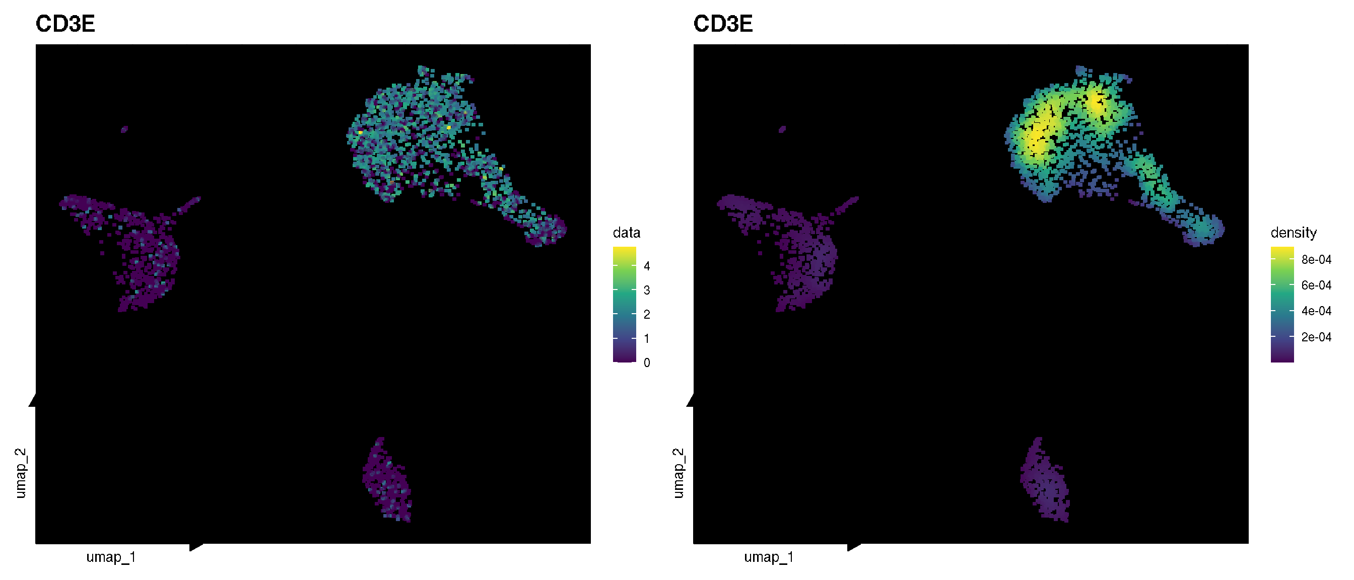
f1 <- sc_feature(pbmc, features = 'CD3E',
                 mapping = aes(bg_colour = ident),
                 geom = geom_bgpoint,
                 density = FALSE,
                 bg_line_width = .4,
                 gap_line_width = .2,
                 size = .5) +
                 scale_color_viridis_c()
f2 <- sc_feature(pbmc, features = 'CD3E',
                 mapping = aes(bg_colour = ident),
                 geom = geom_bgpoint,
                 density = TRUE,
                 bg_line_width = .4,
                 gap_line_width = .22,
                 size = .8) +
         scale_color_viridis_c()

f1 | f2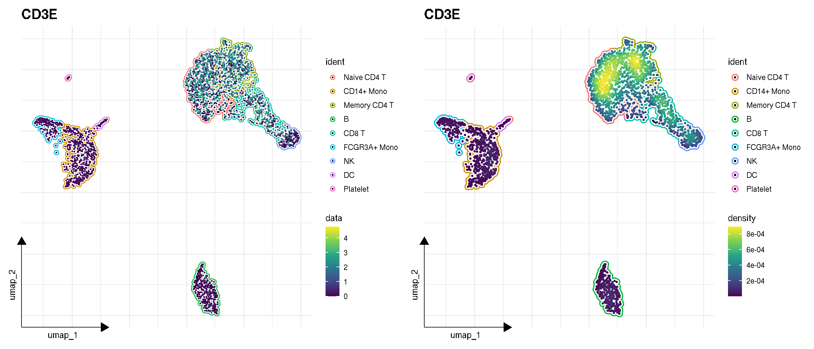

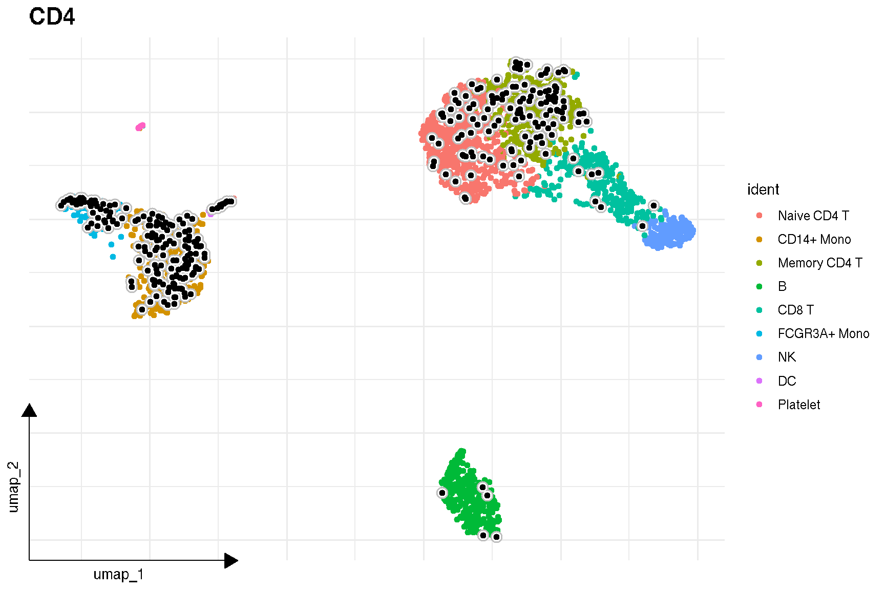
1.4 Visualize selected clusters
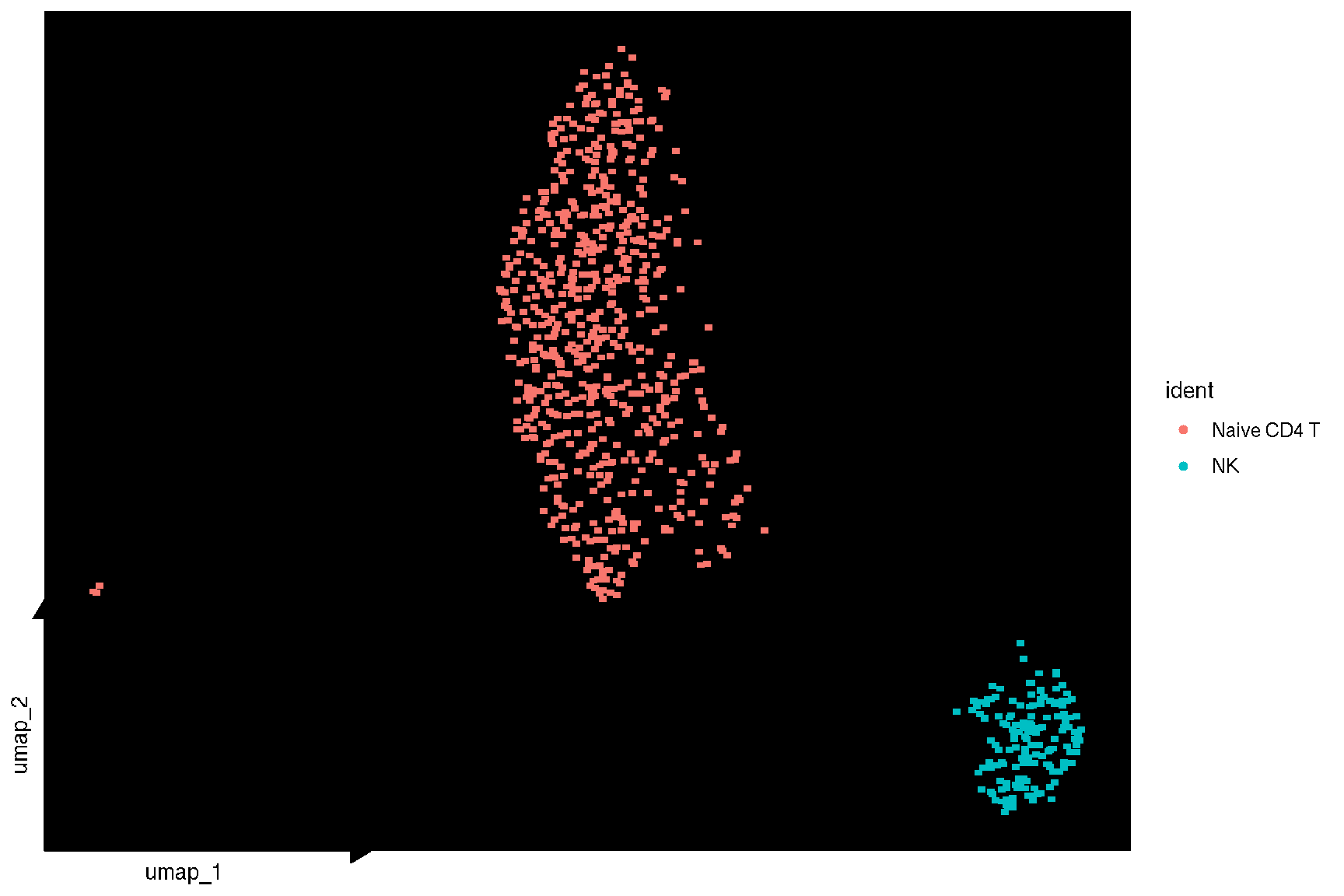
sc_dim(pbmc, color='grey', geom = geom_bgpoint, pointsize=1) +
  sc_dim_geom_sub(subset=selected, mapping = aes(bg_colour = ident)) +
    sc_dim_geom_label(geom = shadowtext::geom_shadowtext,
          mapping = aes(subset = ident %in% selected),
            color='black', bg.color='white')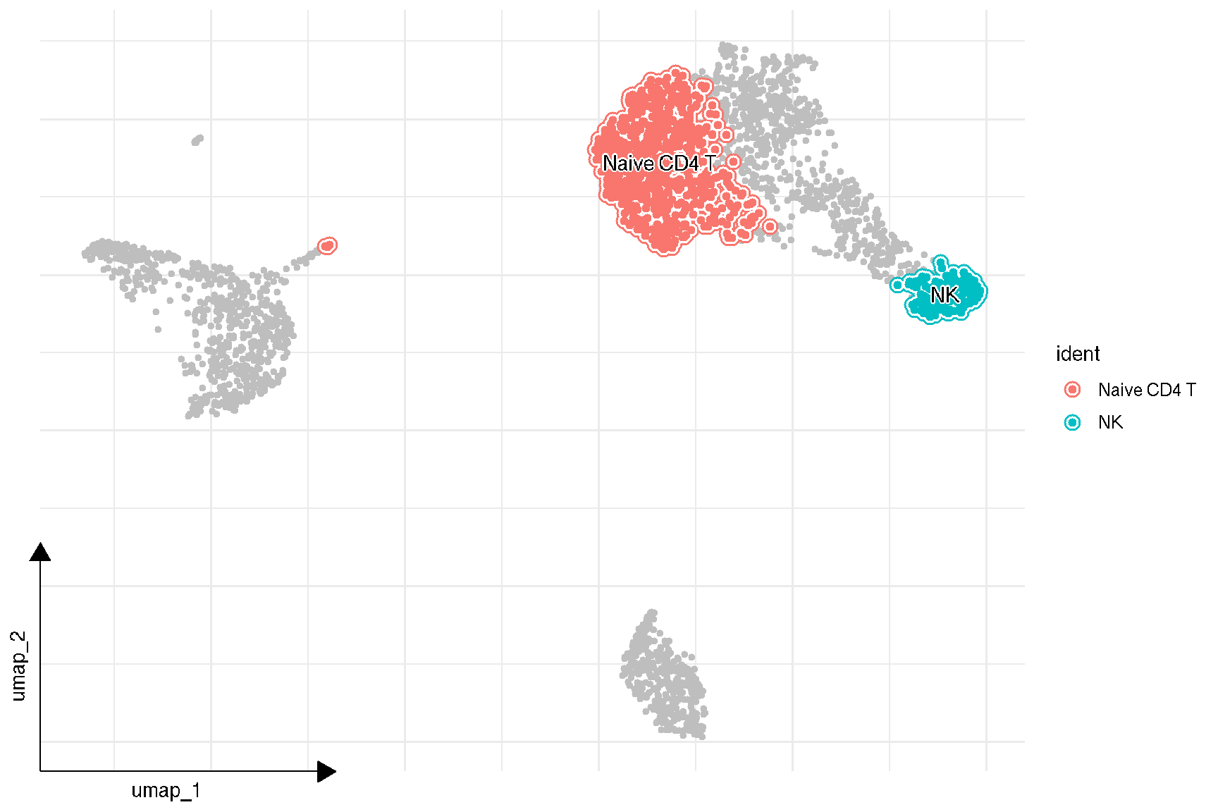
1.5 Dot plot for selected features
features = c("MS4A1", "GNLY", "CD3E",
            "CD14", "FCER1A", "FCGR3A",
            "LYZ", "PPBP", "CD8A")
# DotPlot(pbmc, features = features,
#        group.by = 'seurat_clusters')

sc_dot(pbmc, features=features)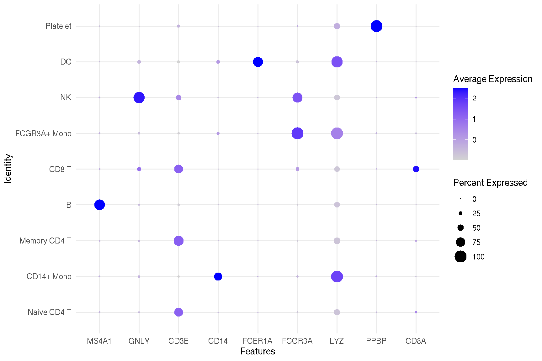
1.6 Violin plot of gene expression
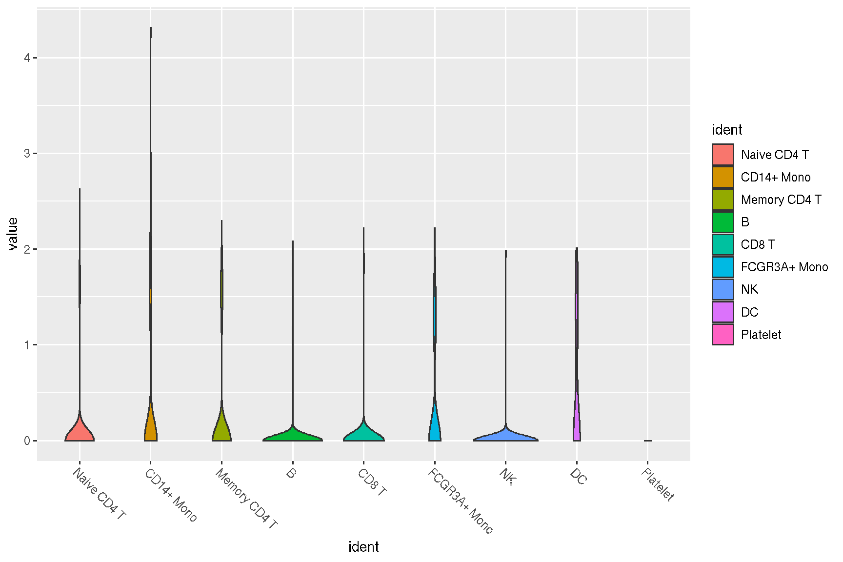
## allows applying an user-defined function to transform/filter the data
sc_violin(pbmc, 'CD4', .fun=function(d) dplyr::filter(d, value > 0)) +
  ggforce::geom_sina(size=.1) +
  guides(x = guide_axis(angle = -45))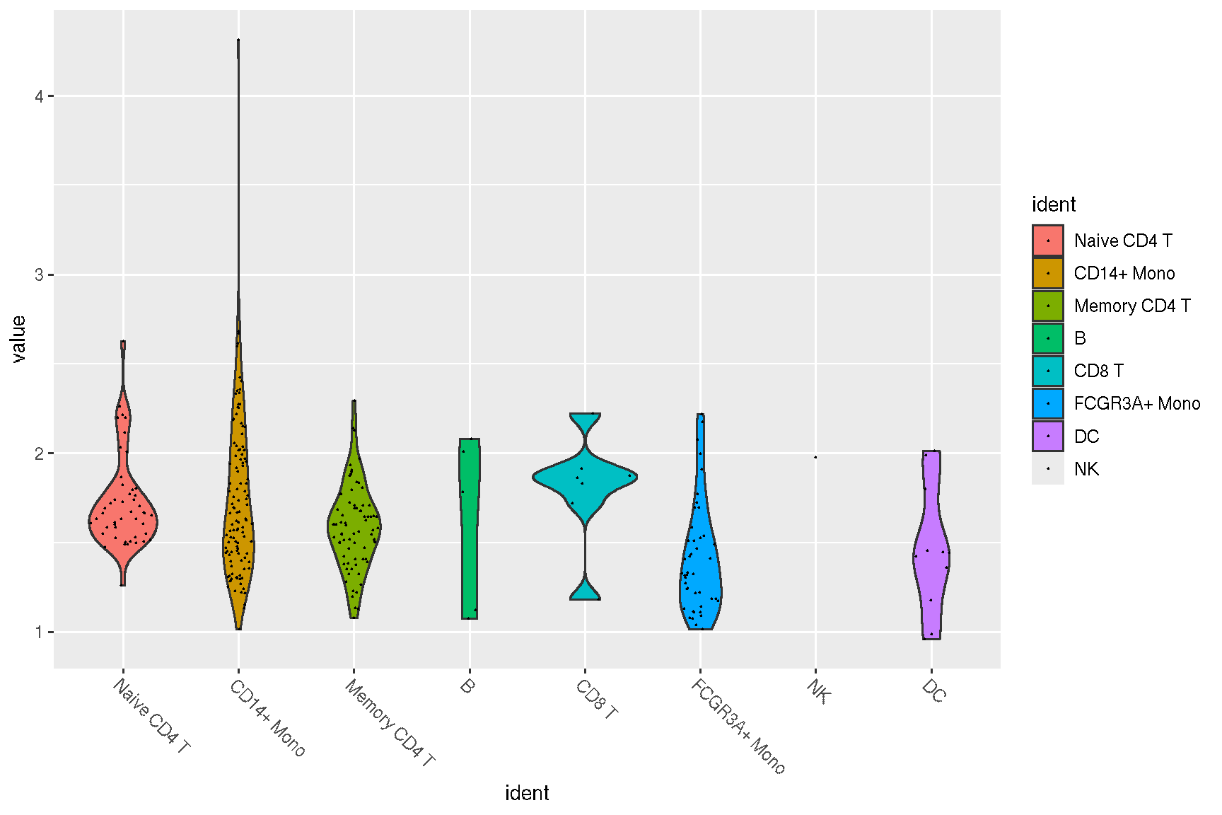
#VlnPlot(pbmc, features)
sc_violin(pbmc, features) +
  theme(axis.text.x = element_text(angle=45, hjust=1))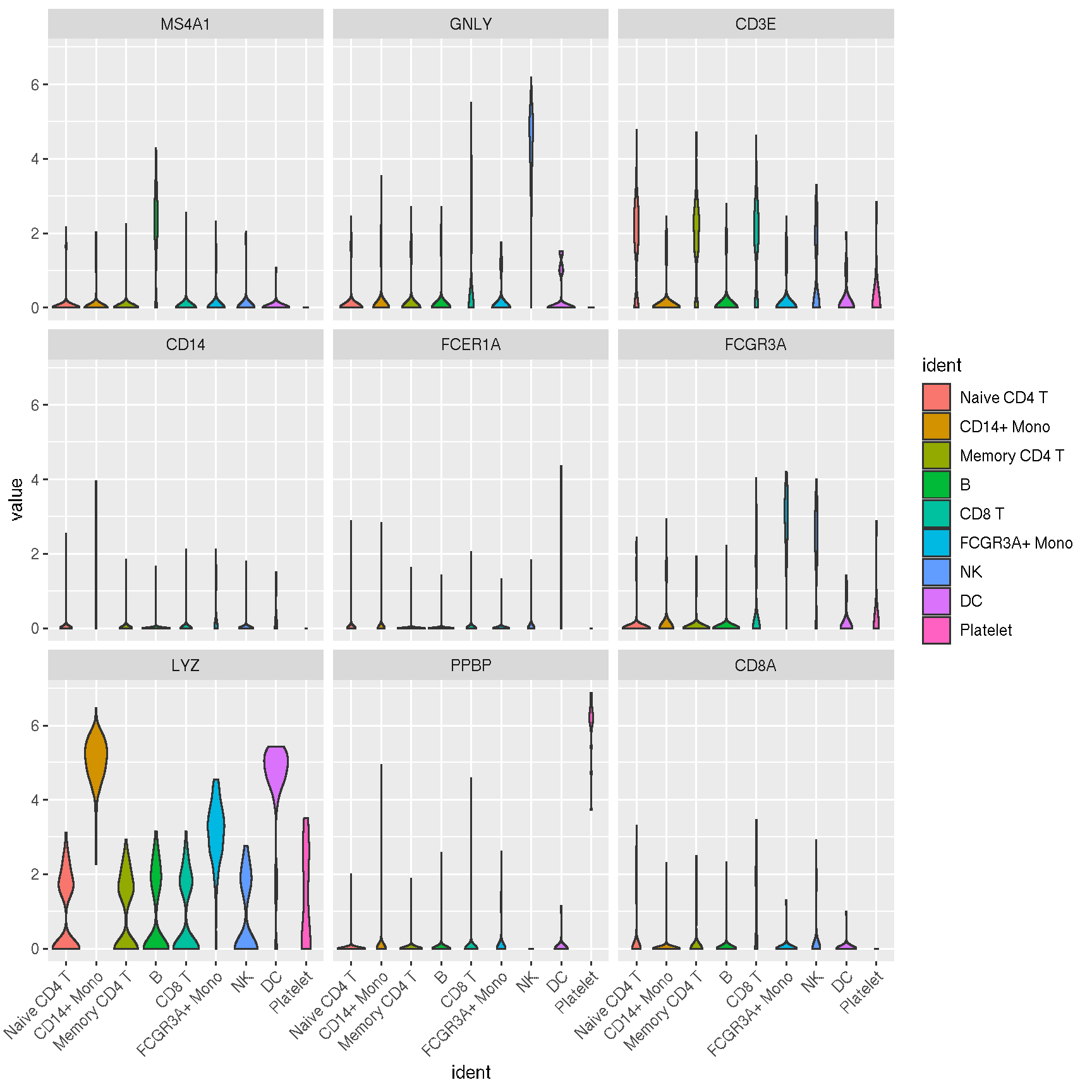
1.7 Spatial features
library(SeuratData)
if (!requireNamespace("SVP", quietly=TRUE)){
    remotes::install_github("YuLab-SMU/SVP")
}
# InstallData("stxBrain")
brain <- LoadData("stxBrain", type = "anterior1")
# Normalization
brain <- SCTransform(brain, assay = "Spatial", verbose = FALSE)
## SpatialFeaturePlot(brain, features = c("Hpca", "Ttr"))
f1 <- sc_spatial(brain, features = c("Hpca", "Ttr"), image.mirror.axis = 'v', geom = geom_bgpoint, pointsize=1.5)
f2 <- sc_spatial(brain, features=c("Hpca", "Ttr"), image.mirror.axis='v', density=TRUE, geom=geom_bgpoint, pointsize=1.5)
plot_list(f1, f2, ncol=1)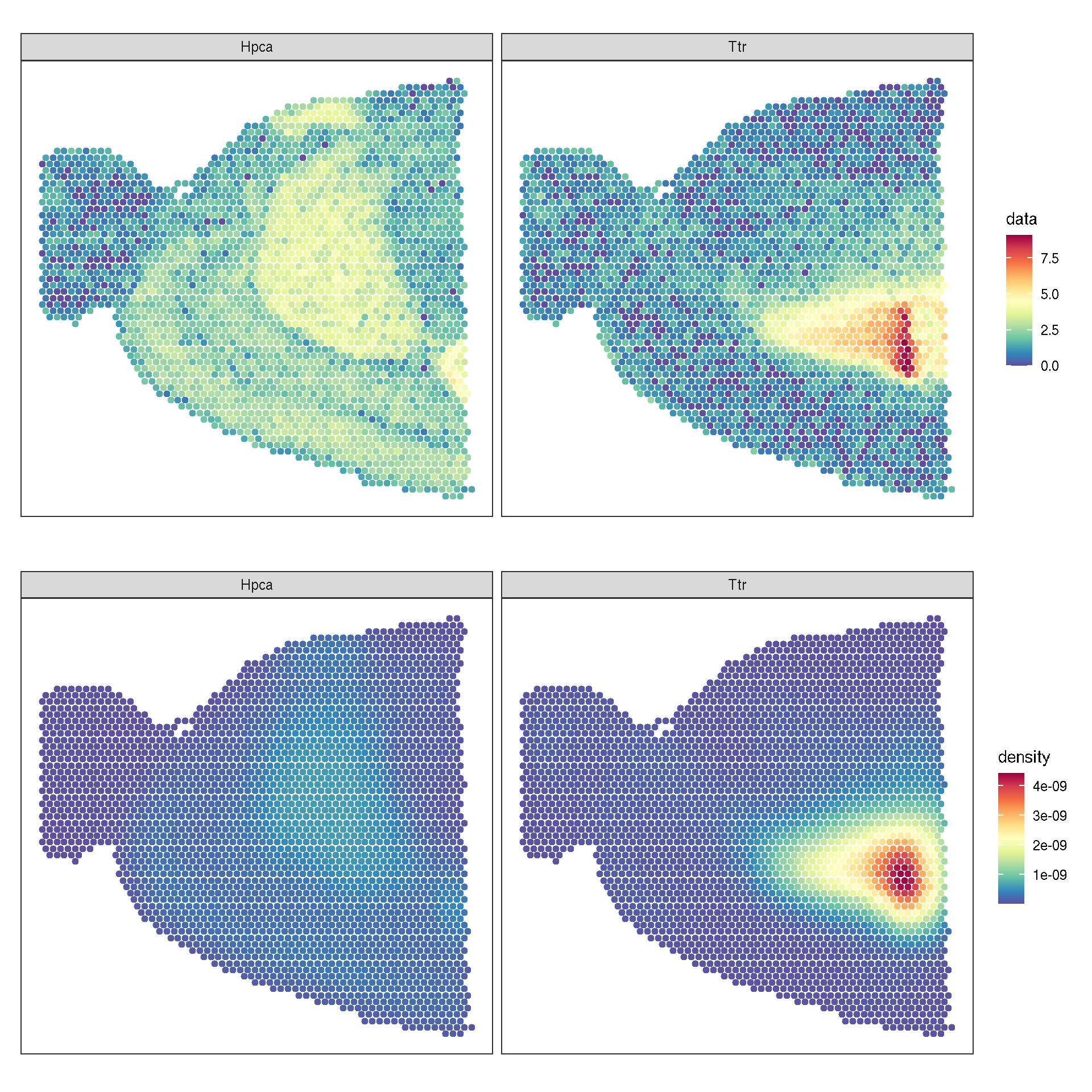
{library(SingleCellExperiment)
library(SpatialExperiment)} |> suppressPackageStartupMessages()
spe.brain <- brain |> as.SingleCellExperiment()
spe.brain <- as(spe.brain, "SpatialExperiment")
spatialCoords(spe.brain) <- GetTissueCoordinates(brain)[,seq(2)] |> as.matrix()
spe.brain
## class: SpatialExperiment
## dim: 17668 2696
## metadata(0):
## assays(2): counts logcounts
## rownames(17668): Xkr4 Sox17 ... CAAA01118383.1
## CAAA01147332.1
## rowData names(0):
## colnames(2696): AAACAAGTATCTCCCA-1 AAACACCAATAACTGC-1
## ... TTGTTTCACATCCAGG-1 TTGTTTCCATACAACT-1
## colData names(9): orig.ident nCount_Spatial ... ident
## sample_id
## reducedDimNames(0):
## mainExpName: SCT
## altExpNames(1): Spatial
## spatialCoords names(2) : x y
## imgData names(0):library(SVP)
res.lisa1 <- runLISA(spe.brain, features = c("Hpca", "Ttr"), assay.type = 'logcounts', weight.method='knn', k=20)
da.lisa1 <- res.lisa1 |> lapply(function(x)x |> tibble::rownames_to_column(var='.BarcodeID')) |> dplyr::bind_rows(.id='features')
head(da.lisa1)## features .BarcodeID Gi E.Gi
## 1 Hpca AAACAAGTATCTCCCA-1 0.0002755991 0.0003710575
## 2 Hpca AAACACCAATAACTGC-1 0.0001295473 0.0003710575
## 3 Hpca AAACAGAGCGACTCCT-1 0.0004076927 0.0003710575
## 4 Hpca AAACAGCTTTCAGAAG-1 0.0001373926 0.0003710575
## 5 Hpca AAACAGGGTCTATATT-1 0.0001222717 0.0003710575
## 6 Hpca AAACATGGTGAGAGGA-1 0.0001670423 0.0003710575
## Var.Gi Z.Gi Pr (z != E(Gi)) cluster.no.test
## 1 1.258174e-09 -2.691186 7.119856e-03 Low
## 2 1.255808e-09 -6.815125 9.418200e-12 Low
## 3 1.259321e-09 1.032357 3.019048e-01 Low
## 4 1.257448e-09 -6.589439 4.414930e-11 Low
## 5 1.255808e-09 -7.020435 2.211781e-12 Low
## 6 1.255808e-09 -5.757061 8.559117e-09 Low
## cluster.test
## 1 Low
## 2 Low
## 3 NoSign
## 4 Low
## 5 Low
## 6 Low# The features and .BarcodeID must be provided
# which be the same to the .BarcodeID and features of
# f1$data
f1 + sc_geom_annot(
data=da.lisa1,
mapping = aes(bg_color=cluster.test, subset=cluster.test=='High'),
pointsize =1.5,
bg_line_width = .3,
gap_line_width=.3,
) +
scale_bg_colour_manual(values = 'black')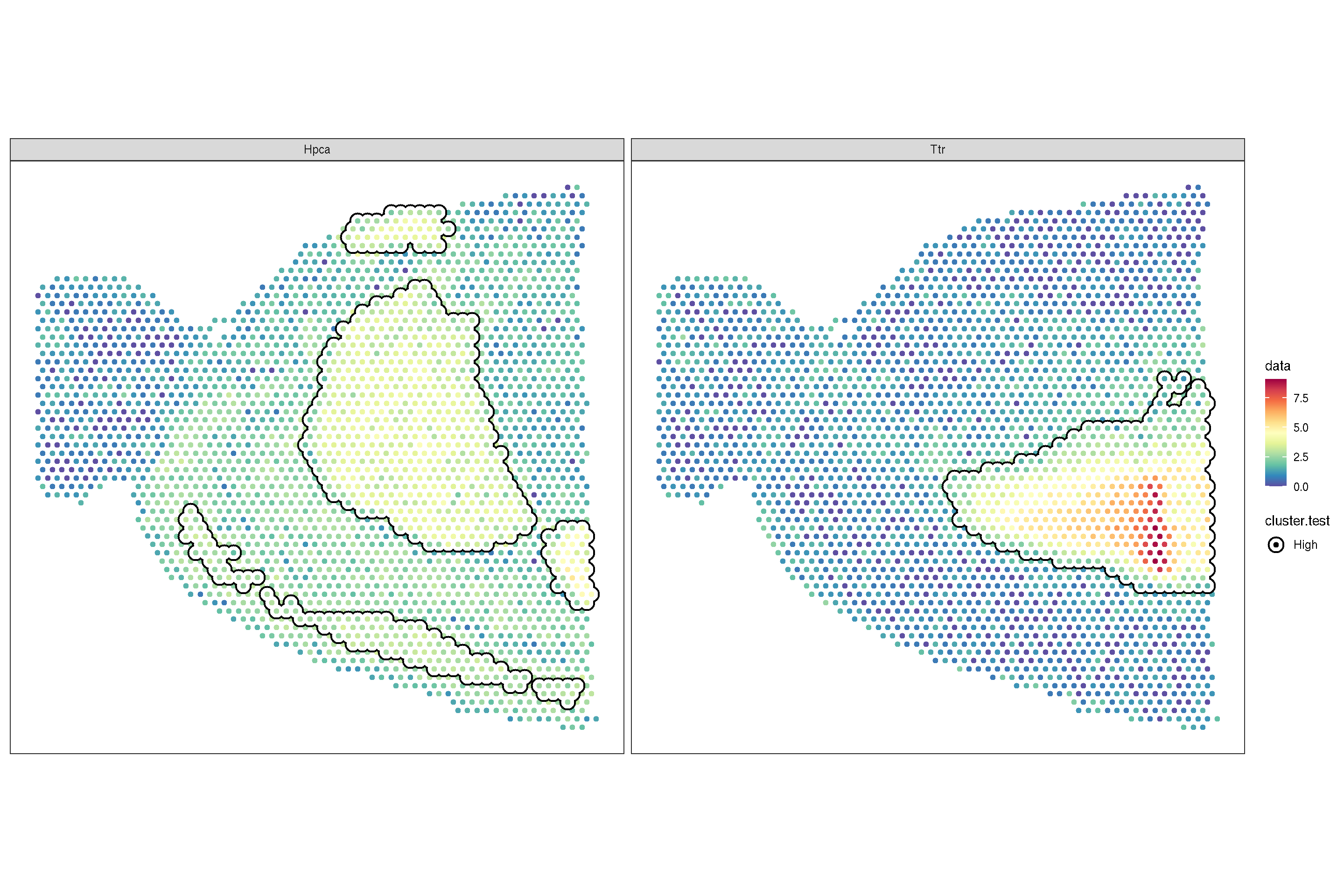
f2 + sc_geom_annot(
        data = da.lisa1,
    mapping = aes(bg_colour = cluster.test, subset = cluster.test == 'High'),
    pointsize = 1.5,
        bg_line_width = .3,
    gap_line_width = .3) +
    scale_bg_colour_manual(values = 'black')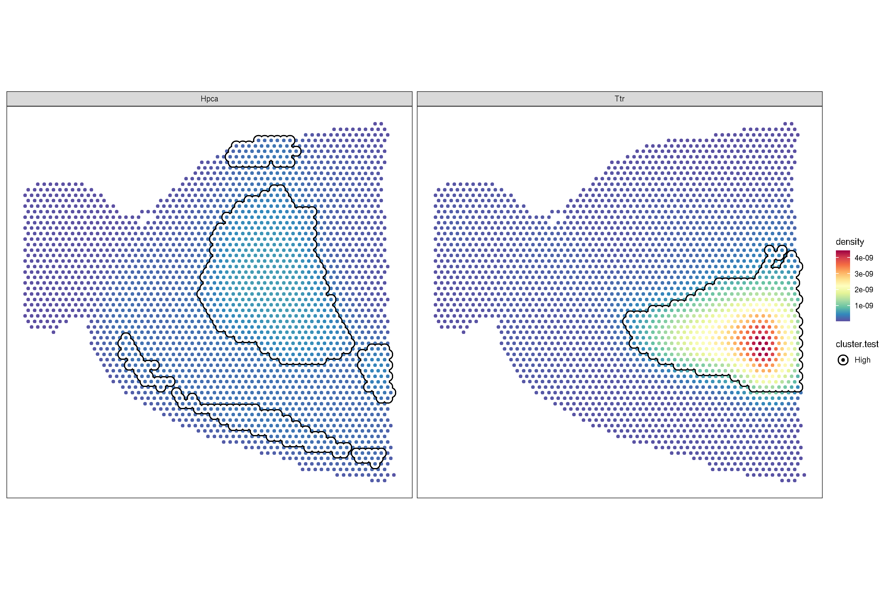
f3 <- sc_spatial(brain, features=c("Hpca", "Ttr"), image.mirror.axis='v',
    density=TRUE, joint=TRUE)
f4 <- sc_spatial(brain, features=c("Hpca", "Ttr"), image.mirror.axis='v',
    density=TRUE, joint=TRUE, common.legend=FALSE)
plot_list(f3, f4, ncol=1)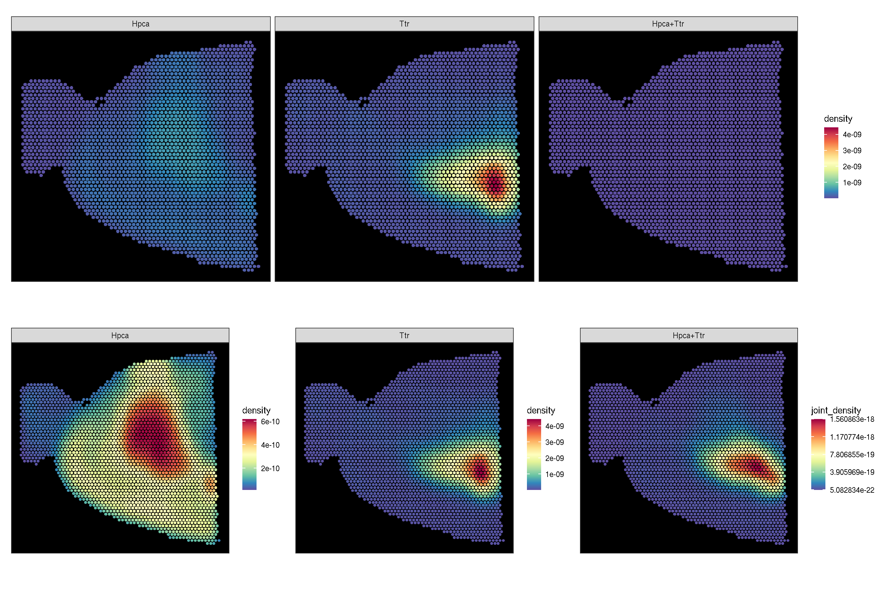
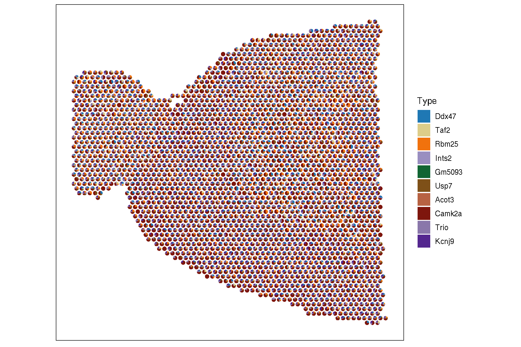
genes <- rownames(brain) |> sample(10)
sc_spatial(brain, features=genes, plot.pie=TRUE,
        pie.radius.scale=.35, image.plot=FALSE,
        color = NA
    )