Workshop of microbiome dataset analysis using MicrobiotaProcess

1. Load required packages

suppressPackageStartupMessages({
    library(MicrobiotaProcess) # an R package for analysis, visualization and biomarker discovery of Microbiome.
    library(phyloseq) # Handling and analysis of high-throughput microbiome census data.
    library(ggplot2) # Create Elegant Data Visualisations Using the Grammar of Graphics.
    library(tidyverse) # Easily Install and Load the 'Tidyverse'.
    library(vegan) # Community Ecology Package.
    library(coin) # Conditional Inference Procedures in a Permutation Test Framework.
    library(reshape2) # Flexibly Reshape Data: A Reboot of the Reshape Package.
    library(ggnewscale) # Multiple Fill and Colour Scales in 'ggplot2'.
})

Here, we use the 43 pediatric IBD stool samples as example, obtained from the Integrative Human Microbiome Project Consortium (iHMP).

2. Importing the output of dada2

The datasets were obtained from https://www.microbiomeanalyst.ca/MicrobiomeAnalyst/resources/data/ibd_data.zip. It contains ibd_asv_table.txt, which is feature table (row features X column samples), ibd_meta.csv, which is metadata file of samples, and ibd_taxa.txt, which is the taxonomic annotation of features. In the session, we use import_dada2 of MicrobiotaProcess to import the datasets, and return a phyloseq object.

library(MicrobiotaProcess)
library(phyloseq)
otuda <- read.table("./IBD_data/ibd_asv_table.txt", header=T, 
                    check.names=F, comment.char="", row.names=1, sep="\t")
# building the output format of removeBimeraDenovo of dada2
otuda <- data.frame(t(otuda), check.names=F)
sampleda <- read.csv("./IBD_data/ibd_meta.csv", row.names=1, comment.char="")
taxda <- read.table("./IBD_data/ibd_taxa.txt", header=T, 
                    row.names=1, check.names=F, comment.char="")
# the feature names should be the same with rownames of taxda. 
taxda <- taxda[match(colnames(otuda), rownames(taxda)),]
psraw <- import_dada2(seqtab=otuda, taxatab=taxda, sampleda=sampleda)
# view the reads depth of samples. In this example, 
# we remove the sample contained less than 20914 otus.
# sort(rowSums(otu_table(psraw)))

# samples were removed, which the reads number is too little.
psraw <- prune_samples(sample_sums(psraw)>=sort(rowSums(otu_table(psraw)))[3], psraw)
# then the samples were rarefied to 20914 reads.
set.seed(1024)
ps <- rarefy_even_depth(psraw)
ps
#> phyloseq-class experiment-level object
#> otu_table()   OTU Table:         [ 1432 taxa and 41 samples ]
#> sample_data() Sample Data:       [ 41 samples by 1 sample variables ]
#> tax_table()   Taxonomy Table:    [ 1432 taxa by 7 taxonomic ranks ]
#> refseq()      DNAStringSet:      [ 1432 reference sequences ]

2.1 Other import

List of import function

Package	Import Function	Description
MicrobiotaProcess	import_qiime2	Import function to load the output of qiime2
phyloseq	import_biom	Import phyloseq data from biom-format file
	import_qiime	Import function to read the now legacy-format QIIME OTU table
	import_RDP_otu	Import new RDP OTU-table format
	import_uparse	Import UPARSE file format
	import_mothur	General function for importing mothur data files into phyloseq
base	read.table or read.csv	import table

# We also can use phyloseq to build phyloseq object.
library(phyloseq)
ps2 <- phyloseq(otu_table(otuda, taxa_are_rows=FALSE), sample_data(sampleda), tax_table(as.matrix(taxda)))
ps2

output

#> phyloseq-class experiment-level object
#> otu_table()   OTU Table:         [ 1681 taxa and 43 samples ]
#> sample_data() Sample Data:       [ 43 samples by 1 sample variables ]
#> tax_table()   Taxonomy Table:    [ 1681 taxa by 7 taxonomic ranks ]

3. alpha diversity analysis

3.1 rarefaction visualization

Rarefaction, based on sampling technique, was used to compensate for the effect of sample size on the number of units observed in a sample. MicrobiotaProcess provided ggrarecurve to plot the curves, based on rrarefy of vegan

library(MicrobiotaProcess)
library(patchwork)
# for reproducibly random number
set.seed(1024)
rareres <- get_rarecurve(obj=ps, chunks=400)

p_rare <- ggrarecurve(obj=rareres,
                      indexNames=c("Observe","Chao1","ACE"),
                      ) +
          theme(legend.spacing.y=unit(0.01,"cm"),
                legend.text=element_text(size=4))

prare1 <- ggrarecurve(obj=rareres, factorNames="Group",
                      indexNames=c("Observe", "Chao1", "ACE")
                      ) +
          scale_fill_manual(values=c("#00AED7", "#FD9347"))+
          scale_color_manual(values=c("#00AED7", "#FD9347"))+
          theme_bw()+
          theme(axis.text=element_text(size=8), panel.grid=element_blank(),
                strip.background = element_rect(colour=NA,fill="grey"),
                strip.text.x = element_text(face="bold"))          

prare2 <- ggrarecurve(obj=rareres,
                      factorNames="Group",
                      shadow=FALSE,
                      indexNames=c("Observe", "Chao1", "ACE")
                      ) +
          scale_color_manual(values=c("#00AED7", "#FD9347"))+
          theme_bw()+
          theme(axis.text=element_text(size=8), panel.grid=element_blank(),
                strip.background = element_rect(colour=NA,fill="grey"),
                strip.text.x = element_text(face="bold"))
p_rare / prare1 / prare2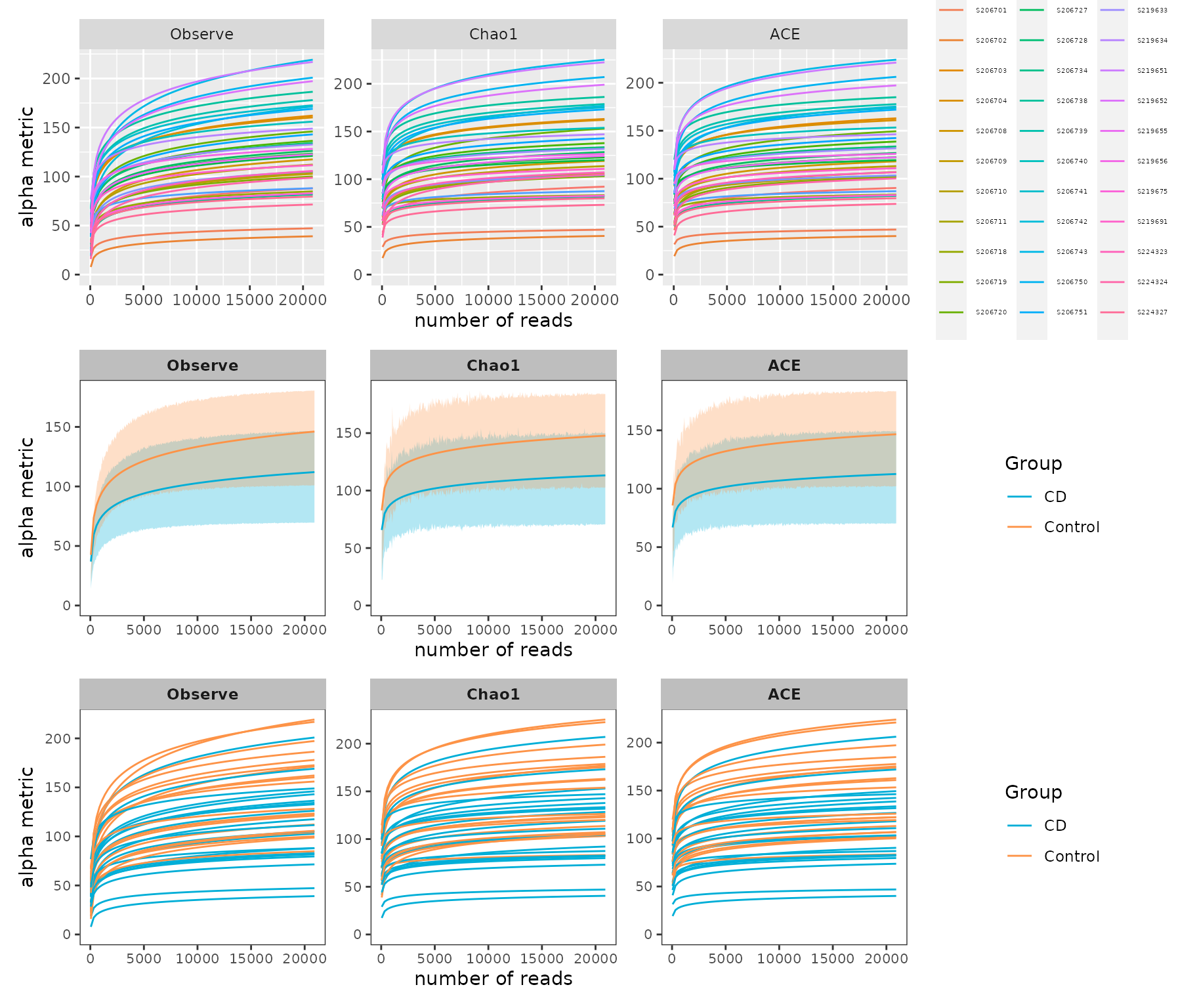

Example of rarefaction curve of samples

Since the curves in each sample were near saturation, the sequencing data were great enough with very few new species undetected

3.2 Calculation and different analysis of alpha index

Alpha index can evaluate the richness and abundance of microbial communities. MicrobiotaProcess provides get_alphaindex to calculate alpha index. Six common diversity measures (Observe, Chao1, ACE, Shannon, Simpson, J) are supported. And the different groups of samples can be tested and visualize by ggbox.

library(MicrobiotaProcess)
alphaobj <- get_alphaindex(ps)
head(as.data.frame(alphaobj))
#>         Observe    Chao1       ACE  Shannon   Simpson         J   Group
#> S206700      86  93.0000  90.13504 2.868408 0.8911390 0.6439570      CD
#> S206701      45  45.0000  45.00000 1.634528 0.5614782 0.4293861      CD
#> S206702      38  39.5000  39.31896 0.509799 0.1502078 0.1401476      CD
#> S206703     156 157.6667 157.89265 3.507910 0.9104597 0.6946554 Control
#> S206704     155 160.0000 157.08120 3.946515 0.9642167 0.7825068 Control
#> S206708     113 118.0000 114.51622 2.747711 0.8443571 0.5812324      CD

p_alpha <- ggbox(alphaobj, geom="violin", factorNames="Group") +
           scale_fill_manual(values=c("#00AED7", "#FD9347"))+
           theme(strip.background = element_rect(colour=NA, fill="grey"))
p_alpha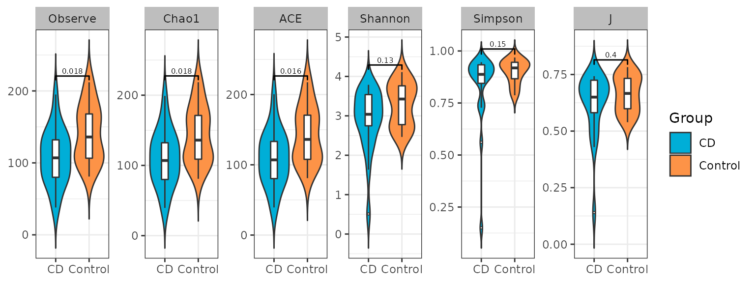

Example of alpha box of samples

4. Taxonomy composition analysis

4.1 Statistics and visualization of specific levels

MicrobiotaProcess presents the ggbartax for the visualization of composition of microbial communities. If you want to get the abundance of specific levels of class, You can use get_taxadf then use ggbartax to visualize.

library(ggplot2)
library(MicrobiotaProcess)

classtaxa <- get_taxadf(obj=ps, taxlevel=3)
# The 30 most abundant taxonomy will be visualized by default (parameter `topn=30`). 
pclass <- ggbartax(obj=classtaxa, facetNames="Group") +
          xlab(NULL) +
          ylab("relative abundance (%)") +
          scale_fill_manual(values=c(colorRampPalette(RColorBrewer::brewer.pal(12,"Set3"))(31))) +
          guides(fill= guide_legend(keywidth = 0.5, keyheight = 0.5))
pclass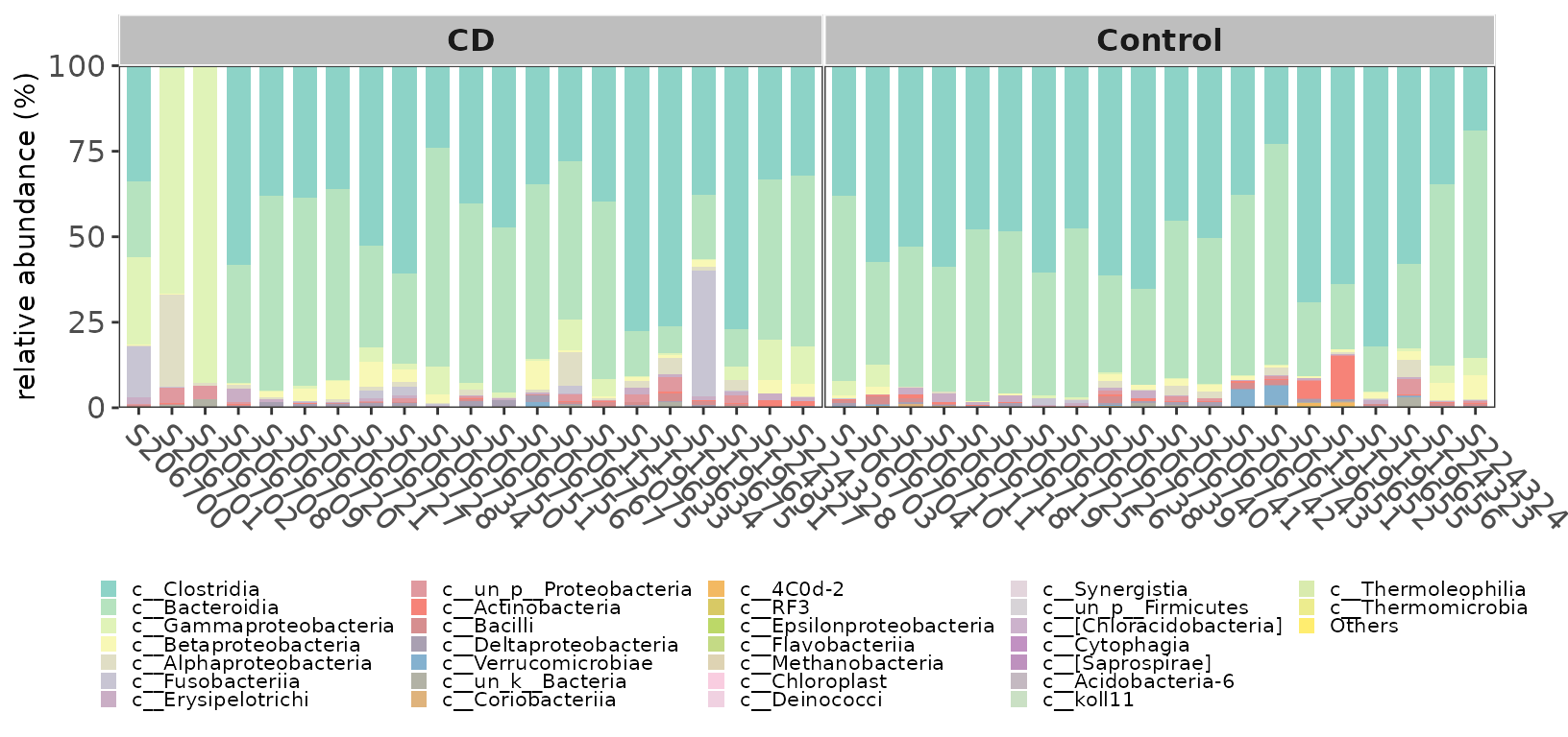

Example of taxonomic abundance of samples

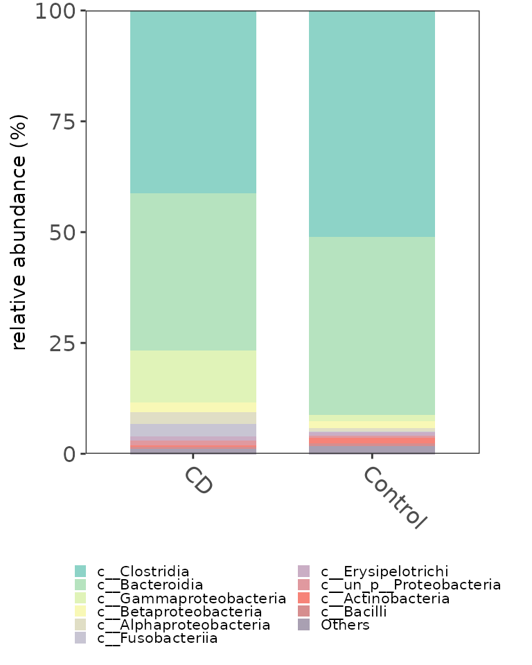
# Show the abundance in different groups.
fclass <- ggbartax(obj=classtaxa, facetNames="Group", plotgroup=TRUE, topn=10) +
          xlab(NULL) +
          ylab("relative abundance (%)") +
          scale_fill_manual(values=c(colorRampPalette(RColorBrewer::brewer.pal(12,"Set3"))(31))) +
          guides(fill= guide_legend(keywidth = 0.5, keyheight = 0.5, ncol=2))
fclass

plot

If you want to view the count of taxonomy, you can set the count parameter of ggbartax to TRUE.

pclass2 <- ggbartax(obj=classtaxa, count=TRUE, facetNames="Group") +
          xlab(NULL) +
          ylab("count reads") +
          scale_fill_manual(values=c(colorRampPalette(RColorBrewer::brewer.pal(12,"Set3"))(31))) +
          guides(fill= guide_legend(keywidth = 0.5, keyheight = 0.5))
pclass2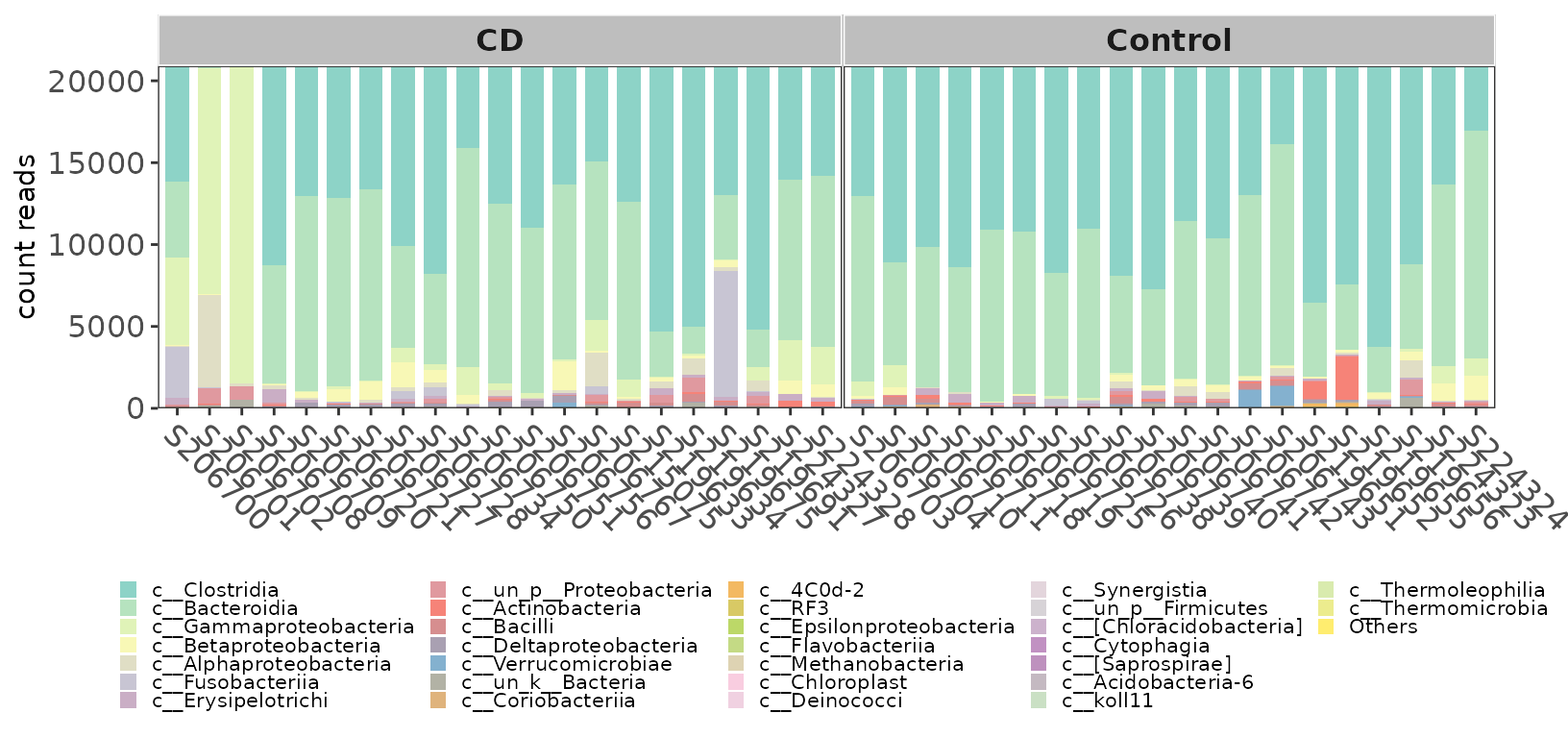

Example of taxonomic abundance (Count) of samples

4.2 Venn or Upset plot

The Venn or UpSet plot can help us to obtain the difference between groups in overview. MicrobiotaProcess provides features to obtain the input of VennDiagram or UpSet package.

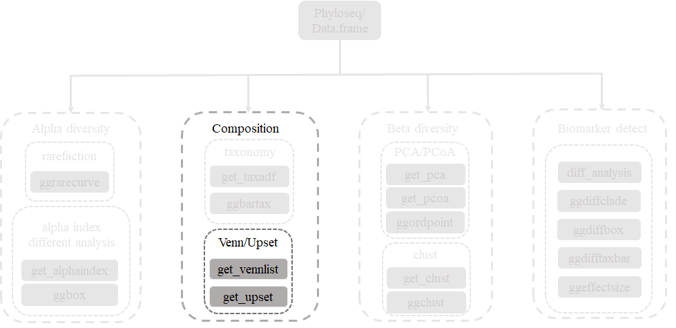
vennlist <- get_vennlist(obj=ps, factorNames="Group")
upsetda <- get_upset(obj=ps, factorNames="Group")
library(VennDiagram)
library(UpSetR)
vennp <- venn.diagram(vennlist,
                      height=5,
                      width=5, 
                      filename=NULL, 
                      fill=c("#00AED7", "#FD9347"),
                      cat.col=c("#00AED7", "#FD9347"),
                      alpha = 0.85, 
                      fontfamily = "serif",
                      fontface = "bold",
                      cex = 1.2,
                      cat.cex = 1.3,
                      cat.default.pos = "outer",
                      cat.dist=0.1,
                      margin = 0.1, 
                      lwd = 3,
                      lty ='dotted',
                      imagetype = "svg")
grid::grid.draw(vennp)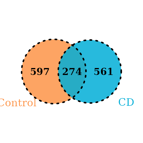

Example of Venn plot

upset(upsetda, sets=unique(as.vector(sample_data(ps)$Group)), 
      sets.bar.color = "#56B4E9",
      order.by = "freq", 
      empty.intersections = "on")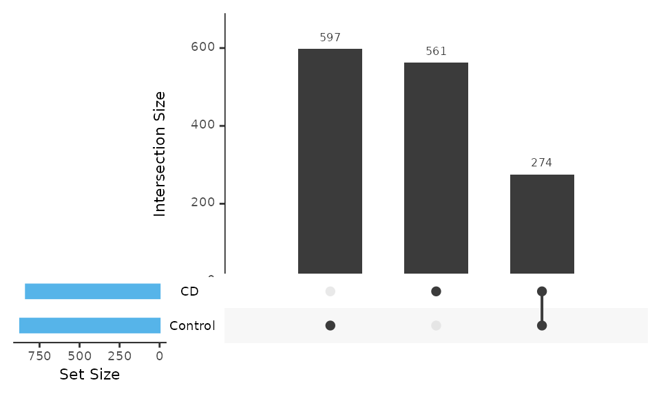

Example of Upset plot

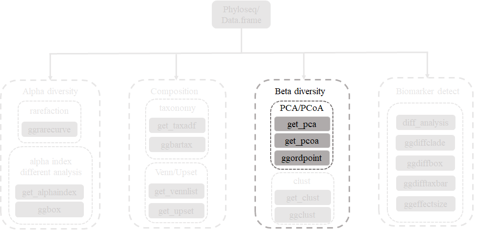
5. beta analysis

5.1 PCA analysis

PCA (Principal component analysis) and PCoA (Principal Coordinate Analysis) are general statistical procedures to compare groups of samples. And PCoA can based on the phylogenetic or count-based distance metrics, such as Bray-Curtis, Jaccard, Unweighted-UniFrac and weighted-UniFrac. MicrobiotaProcess presents the get_pca, get_pcoa and ggordpoint for the analysis.

library(MicrobiotaProcess)
library(patchwork)
# If the input was normalized, the method parameter should be setted NULL.
pcares <- get_pca(obj=ps, method="hellinger")
# Visulizing the result
pcaplot1 <- ggordpoint(obj=pcares, biplot=TRUE, speciesannot=TRUE,
                      factorNames=c("Group"), ellipse=TRUE) +
            scale_color_manual(values=c("#00AED7", "#FD9347")) +
            scale_fill_manual(values=c("#00AED7", "#FD9347"))
# pc = c(1, 3) to show the first and third principal components.
pcaplot2 <- ggordpoint(obj=pcares, pc=c(1, 3), biplot=TRUE, speciesannot=TRUE,
                       factorNames=c("Group"), ellipse=TRUE) +
            scale_color_manual(values=c("#00AED7", "#FD9347")) +
            scale_fill_manual(values=c("#00AED7", "#FD9347"))
pcaplot1 | pcaplot2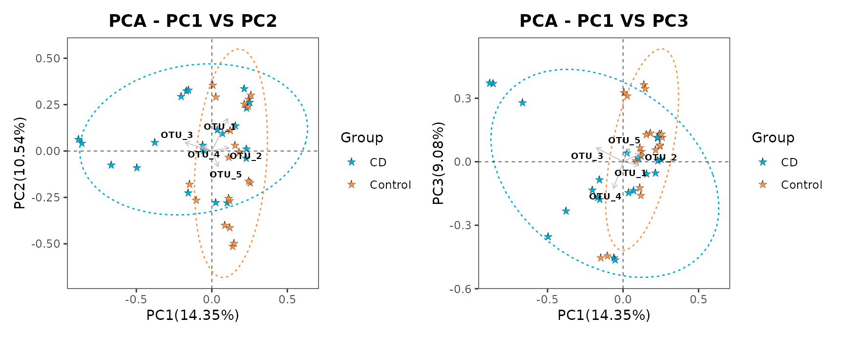

Example of PCA of samples

5.2 PCoA analysis

# distmethod
# "unifrac",  "wunifrac", "manhattan", "euclidean", "canberra", "bray", "kulczynski" ...(vegdist, dist)
pcoares <- get_pcoa(obj=ps, distmethod="bray", method="hellinger")
# Visualizing the result
pcoaplot1 <- ggordpoint(obj=pcoares, biplot=TRUE, speciesannot=TRUE,
                       factorNames=c("Group"), ellipse=TRUE) +
            scale_color_manual(values=c("#00AED7", "#FD9347")) +
            scale_fill_manual(values=c("#00AED7", "#FD9347"))
# first and third principal co-ordinates
pcoaplot2 <- ggordpoint(obj=pcoares, pc=c(1, 3), biplot=TRUE, speciesannot=TRUE,
                        factorNames=c("Group"), ellipse=TRUE) +
             scale_color_manual(values=c("#00AED7", "#FD9347")) +
             scale_fill_manual(values=c("#00AED7", "#FD9347"))
pcoaplot1 | pcoaplot2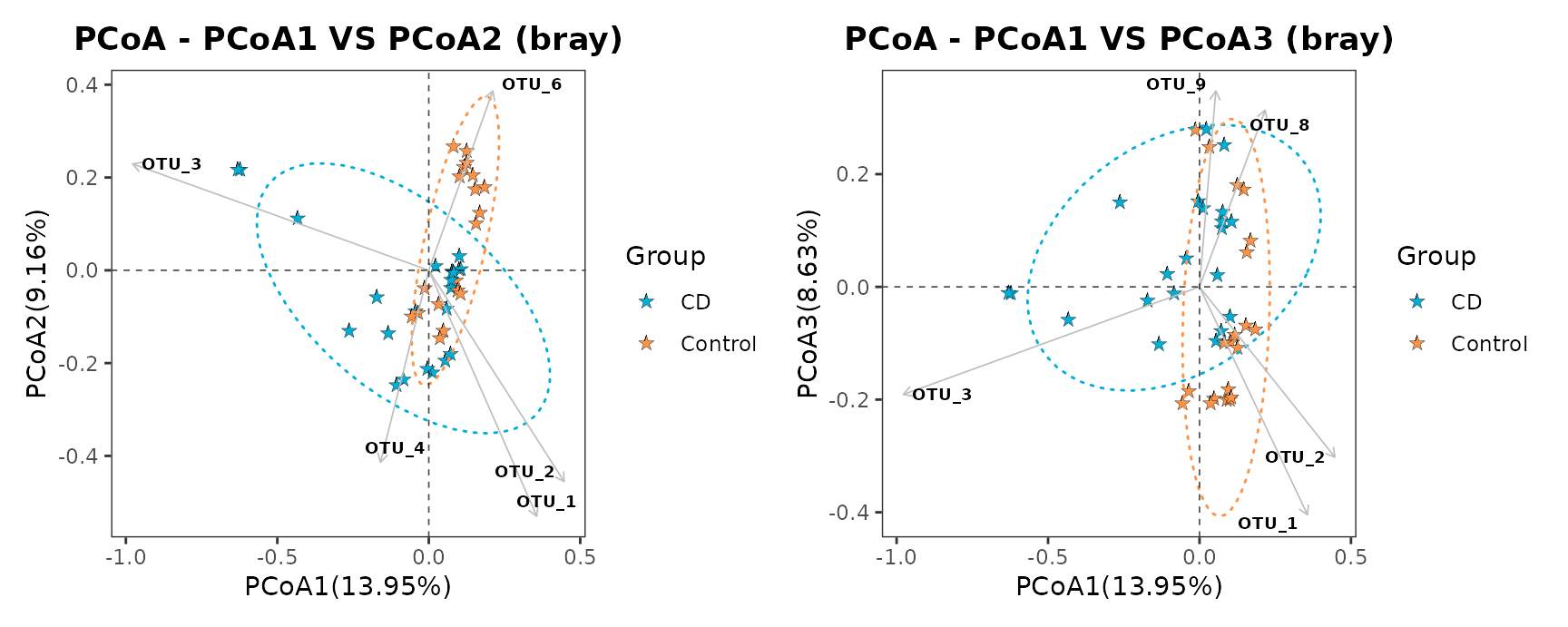

Example of PCoA of samples

5.3 Permutational Multivariate Analysis of Variance

We also can perform the Permutational Multivariate Analysis of Variance using the vegan

distme <- get_dist(ps, distmethod ="bray", method="hellinger")
sampleda <- data.frame(sample_data(ps), check.names=FALSE)
sampleda <- sampleda[match(colnames(as.matrix(distme)),rownames(sampleda)),,drop=FALSE]
sampleda$Group <- factor(sampleda$Group)
set.seed(1024)
adores <- adonis(distme ~ Group, data=sampleda, permutation=9999)
data.frame(adores$aov.tab)

output

#>           Df  SumsOfSqs   MeanSqs  F.Model         R2 Pr..F.
#> Group      1  0.7645291 0.7645291 3.199178 0.07581139  1e-04
#> Residuals 39  9.3200922 0.2389767       NA 0.92418861     NA
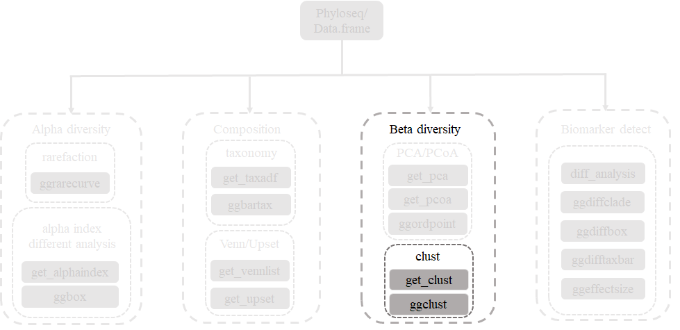
#> Total     40 10.0846214        NA       NA 1.00000000     NA

5.4 hierarchical cluster analysis of samples

beta diversity metrics can assess the differences between microbial communities. It can be visualized with PCA or PCoA, this can also be visualized with hierarchical clustering. MicrobiotaProcess implements the analysis based on ggtree.

library(ggplot2)
library(MicrobiotaProcess)
library(ggtree)
hcsample <- get_clust(obj=ps, distmethod="bray",
                      method="hellinger", hclustmethod="average")
# rectangular layout
cplot1 <- ggclust(obj=hcsample,
                  layout = "rectangular",
                  pointsize=1,
                  fontsize=0,
                  factorNames=c("Group")
              ) +
              scale_color_manual(values=c("#00AED7", "#FD9347")) +
              theme_tree2(legend.position="right",
              plot.title = element_text(face="bold", lineheight=25,hjust=0.5))
# circular layout
cplot2 <- ggclust(obj=hcsample,
                  layout = "circular",
                  pointsize=1,
                  fontsize=2,
                  factorNames=c("Group")
          ) +
          scale_color_manual(values=c("#00AED7", "#FD9347")) +
          theme(legend.position="right")
cplot1 | cplot2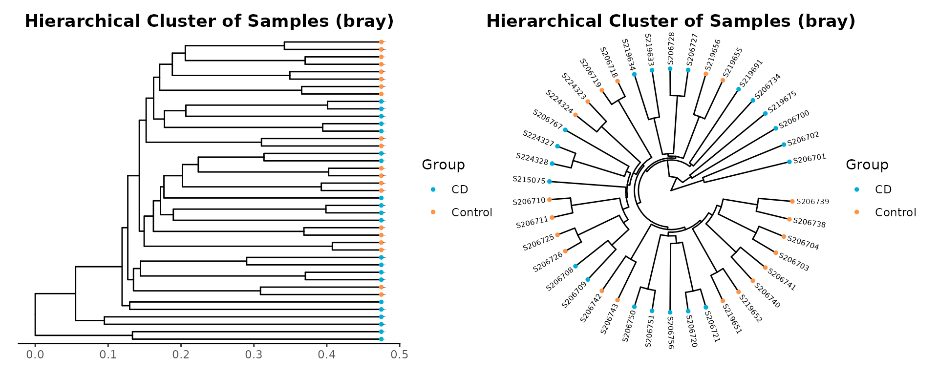

Example of hierarchical clustering of samples

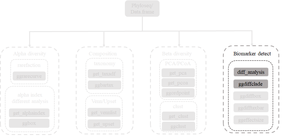
6. biomarker discovery

This package provides diff_analysis to detect the biomarker. And the results can be visualized by ggdiffbox, ggdiffclade, ggeffectsize and ggdifftaxbar

# for the kruskal_test and wilcox_test
library(coin)
library(MicrobiotaProcess)
# Since the effect size was calculated by randomly re-sampling, 
# the seed should be set for reproducibly results.
set.seed(1024)
deres <- diff_analysis(obj = ps, classgroup = "Group",
                       mlfun = "lda",
                       filtermod = "pvalue",
                       firstcomfun = "kruskal_test",
                       firstalpha = 0.05,
                       strictmod = TRUE,
                       secondcomfun = "wilcox_test",
                       subclmin = 3,
                       subclwilc = TRUE,
                       secondalpha = 0.01,
                       lda=3)
deres
#> The original data: 689 features and 41 samples
#> The sample data: 1 variables and 41 samples
#> The taxda contained 1432 by 7 rank
#> after first test (kruskal_test) number of feature (pvalue<=0.05):71
#> after second test (wilcox_test) number of significantly discriminative feature:28
#> after lda, Number of discriminative features: 22 (certain taxonomy classification:15; uncertain taxonomy classication: 7)

6.1 visualization of different results by ggdiffclade

The color of discriminative taxa represent the taxa is more abundant in the corresponding group. The point size shows the negative logarithms (base 10) of pvalue. The bigger size of point shows more significant (lower pvalue), the pvalue was calculated in the first step test.

diffclade_p <- ggdiffclade(
                   obj=deres, 
                   alpha=0.3, 
                   linewd=0.15,
                   skpointsize=0.6, 
                   layout="radial",
                   taxlevel=3, 
                   removeUnkown=TRUE,
                   reduce=TRUE # This argument is to remove the branch of unknown taxonomy.
               ) +
               scale_fill_manual(
                   values=c("#00AED7", "#FD9347")
               ) +
               guides(color = guide_legend(
                                  keywidth = 0.1, 
                                  keyheight = 0.6,
                                  order = 3,
                                  ncol=1)
               ) +
               theme(
                   panel.background=element_rect(fill=NA),
                   legend.position="right", 
                   plot.margin=margin(0,0,0,0),
                   legend.spacing.y=unit(0.02, "cm"), 
                   legend.title=element_text(size=7),
                   legend.text=element_text(size=6), 
                   legend.box.spacing=unit(0.02,"cm")
               )
diffclade_p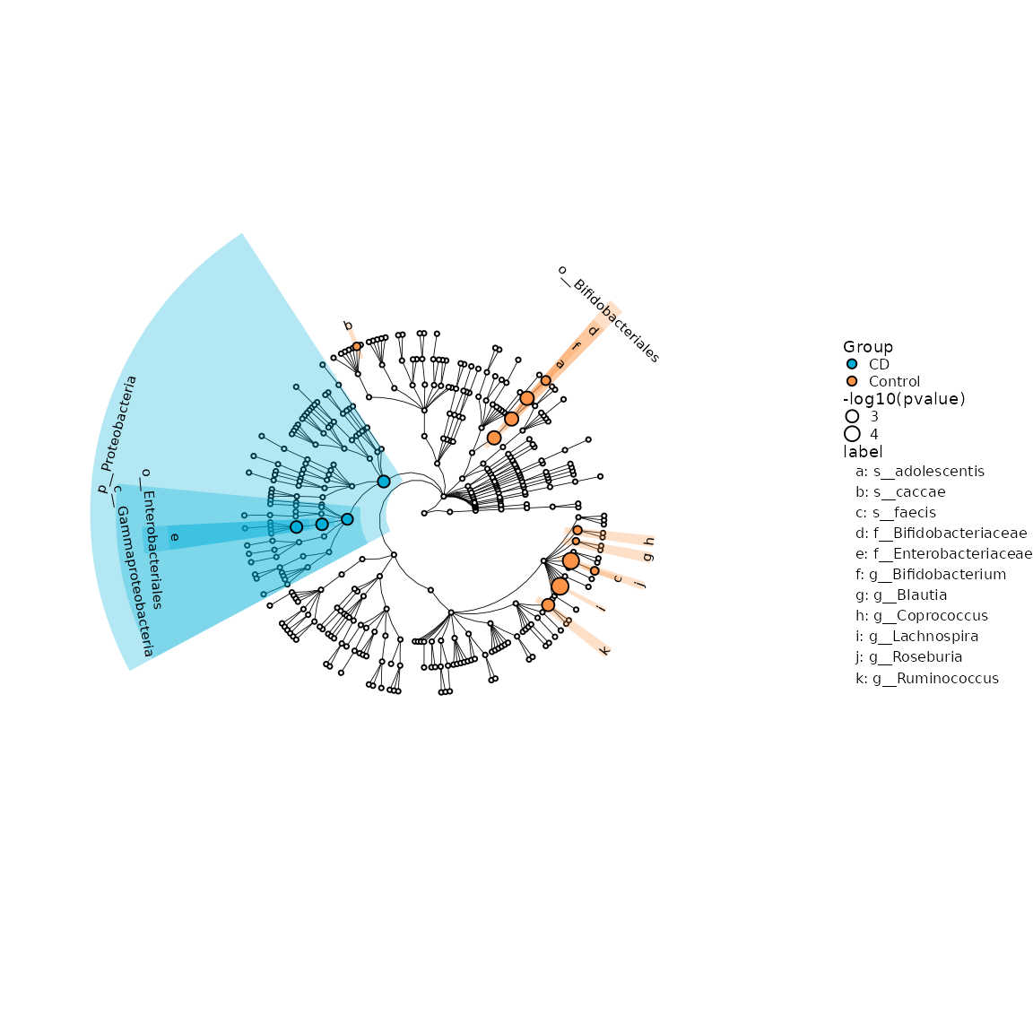

Example of different biomarker clade

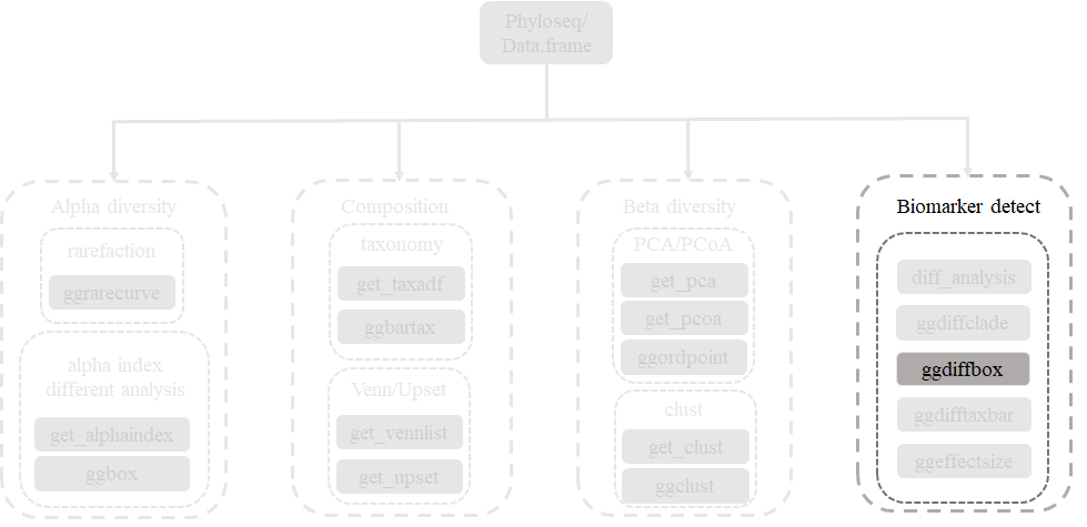
6.2 visualization of different results by ggdiffbox

The left panel represents the relative abundance or abundance (according the standard_method) of biomarker, the right panel represents the confident interval of effect size (LDA or MDA) of biomarker. The bigger confident interval shows that the biomarker is more fluctuant, owing to the influence of samples number.

diffbox <- ggdiffbox(obj=deres, box_notch=FALSE, 
             colorlist=c("#00AED7", "#FD9347"), l_xlabtext="relative abundance")
diffbox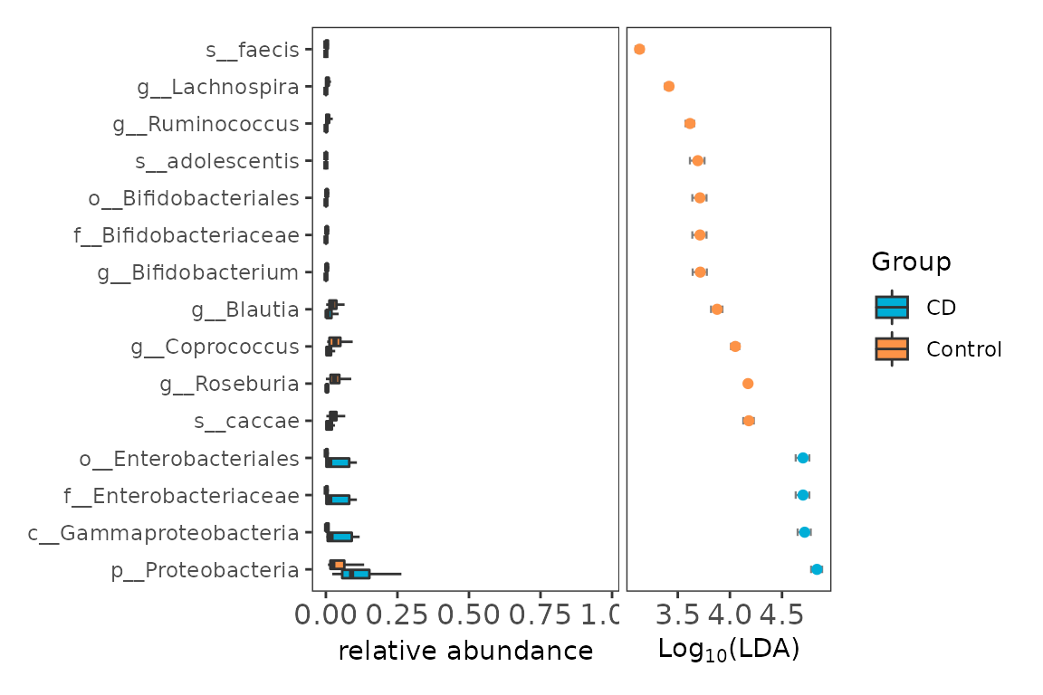

Example of biomarker boxplot and effect size

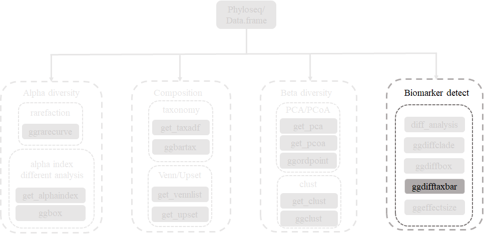
6.3 visualization of different results by ggdifftaxbar

ggdifftaxbar can visualize the abundance of biomarker in each samples of groups, the mean and median abundance of groups or subgroups are also showed. output parameter is the directory of output.

ggdifftaxbar(obj=deres, xtextsize=1.5, 
             output="IBD_biomarkder_barplot",
             coloslist=c("#00AED7", "#FD9347"))

6.4 visualization of different results by ggeffectsize

The result is similar with the result of ggdiffbox, the bigger confident interval shows that the biomarker is more fluctuant owing to the influence of samples number.

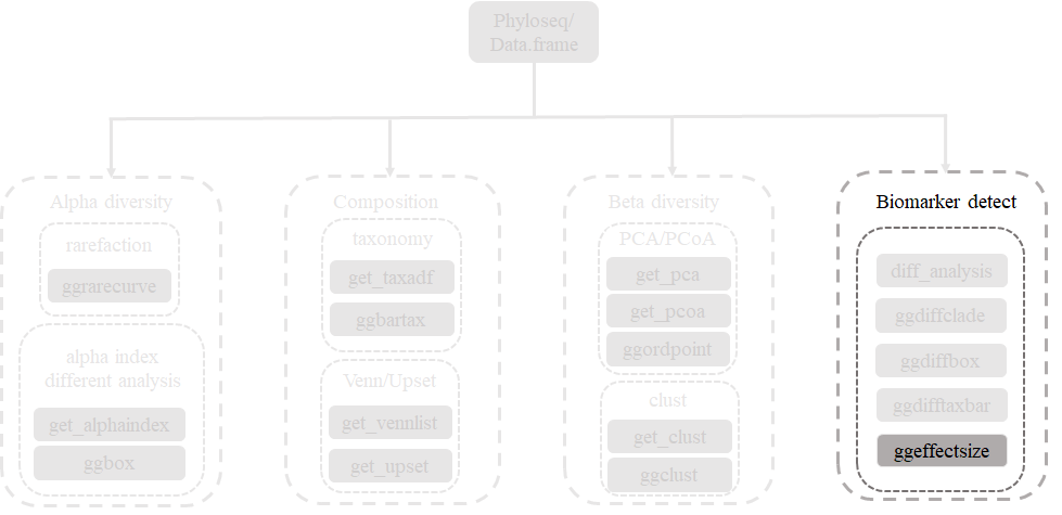
es_p <- ggeffectsize(obj=deres, 
                     lineheight=0.1,
                     linewidth=0.3) + 
        scale_color_manual(values=c("#00AED7", 
                                    "#FD9347")) 

es_p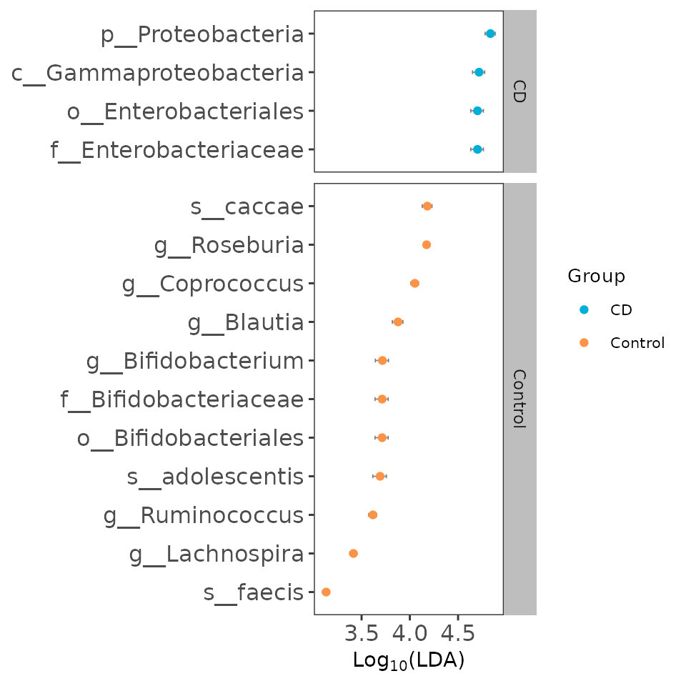

Example of effect size of biomarker

7. Correlation of taxonomy

The result of different analysis also can be visualized with result of correlation.

genustab <- get_taxadf(ps, taxlevel=6)
genustab <- data.frame(t(otu_table(genustab)), check.names=FALSE)
genustab <- data.frame(apply(genustab, 2, function(x)x/sum(x)), check.names=FALSE)

cortest <- WGCNA::corAndPvalue(genustab, method="spearman", alternative="two.sided")
cortest$cor[upper.tri(cortest$cor, diag = TRUE)] <- NA
cortest$p[upper.tri(cortest$p, diag = TRUE)] <- NA
cortab1 <- na.omit(melt(t(cortest$cor))) %>% rename(from=Var1,to=Var2,cor=value)
corptab1 <- na.omit(melt(t(cortest$p))) %>% rename(pvalue=value)
cortab1$fdr <- p.adjust(corptab1$pvalue, method="fdr")

cortab1 <- cortab1 %>% mutate(correlation=case_when(cor>0 ~ "positive",cor < 0 ~ "negative",TRUE ~ "No"))
cortab2 <- cortab1 %>% filter(fdr <= 0.05) %>% filter(cor <= -0.5 | cor >= 0.8)

p <- ggdiffclade(
         obj=deres,
         alpha=0.3,
         linewd=0.25,
         skpointsize=0.2,
         layout="inward_circular",
         taxlevel=7,
         cladetext=0,
         setColors=FALSE,
         xlim=16
     ) +
     scale_fill_manual(values=c("#00AED7", "#FD9347"),
                       guide=guide_legend(keywidth=0.5,
                                          keyheight=0.5,
                                          order=3,
                                          override.aes=list(alpha=1))
     ) +
     scale_size_continuous(range=c(1, 3),
                       guide=guide_legend(keywidth=0.5,keyheight=0.5,order=4,
                                          override.aes=list(shape=21))) +
     scale_colour_manual(values=rep("white", 100),guide="none")

p2 <- p +
      new_scale_color() +
      new_scale("size") +
      geom_tiplab(size=1, hjust=1) +
      geom_taxalink(
          data=cortab2,
          mapping=aes(taxa1=from,
                      taxa2=to,
                      colour=correlation,
                      size=abs(cor)),
          alpha=0.4,
          ncp=10,
          hratio=1,
          offset=1.2
      ) +
      scale_size_continuous(range = c(0.2, 1),
                            guide=guide_legend(keywidth=1, keyheight=0.5,
                                               order=1, override.aes=list(alpha=1))
      ) +
      scale_colour_manual(values=c("chocolate2", "#009E73"),
                          guide=guide_legend(keywidth=0.5, keyheight=0.5,
                          order=2, override.aes=list(alpha=1, size=1)))
p2

plot

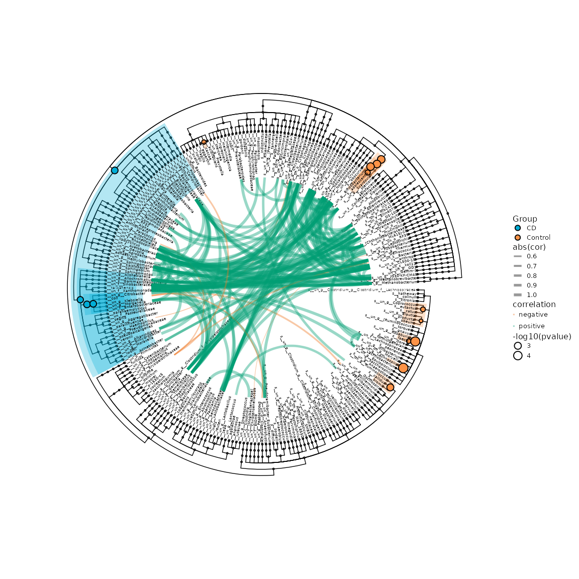
Example of different biomarker clade and correlation of genera

8. Session information

Here is the output of sessionInfo() on the system on which this document was compiled:

output

#> R Under development (unstable) (2020-11-18 r79449)
#> Platform: x86_64-pc-linux-gnu (64-bit)
#> Running under: Ubuntu 20.04.1 LTS
#> 
#> Matrix products: default
#> BLAS/LAPACK: /usr/lib/x86_64-linux-gnu/openblas-pthread/libopenblasp-r0.3.8.so
#> 
#> locale:
#>  [1] LC_CTYPE=en_US.UTF-8       LC_NUMERIC=C              
#>  [3] LC_TIME=en_US.UTF-8        LC_COLLATE=en_US.UTF-8    
#>  [5] LC_MONETARY=en_US.UTF-8    LC_MESSAGES=C             
#>  [7] LC_PAPER=en_US.UTF-8       LC_NAME=C                 
#>  [9] LC_ADDRESS=C               LC_TELEPHONE=C            
#> [11] LC_MEASUREMENT=en_US.UTF-8 LC_IDENTIFICATION=C       
#> 
#> attached base packages:
#> [1] grid      stats     graphics  grDevices utils     datasets  methods  
#> [8] base     
#> 
#> other attached packages:
#>  [1] gdtools_0.2.2           ggtree_2.5.0            UpSetR_1.4.0           
#>  [4] VennDiagram_1.6.20      futile.logger_1.4.3     patchwork_1.1.0        
#>  [7] kableExtra_1.3.1        ggnewscale_0.4.3        reshape2_1.4.4         
#> [10] coin_1.3-1              survival_3.2-7          vegan_2.5-6            
#> [13] lattice_0.20-41         permute_0.9-5           forcats_0.5.0          
#> [16] stringr_1.4.0           dplyr_1.0.2             purrr_0.3.4            
#> [19] readr_1.4.0             tidyr_1.1.2             tibble_3.0.4           
#> [22] tidyverse_1.3.0         ggplot2_3.3.2           phyloseq_1.35.0        
#> [25] MicrobiotaProcess_1.3.2
#> 
#> loaded via a namespace (and not attached):
#>   [1] tidyselect_1.1.0      RSQLite_2.2.1         AnnotationDbi_1.53.0 
#>   [4] htmlwidgets_1.5.2     munsell_0.5.0         preprocessCore_1.53.0
#>   [7] codetools_0.2-18      ragg_0.4.0            withr_2.3.0          
#>  [10] colorspace_2.0-0      Biobase_2.51.0        highr_0.8            
#>  [13] knitr_1.30            rstudioapi_0.13       stats4_4.1.0         
#>  [16] ggsignif_0.6.0        labeling_0.4.2        bit64_4.0.5          
#>  [19] farver_2.0.3          rhdf5_2.35.0          rprojroot_2.0.2      
#>  [22] vctrs_0.3.5           treeio_1.15.1         generics_0.1.0       
#>  [25] TH.data_1.0-10        lambda.r_1.2.4        xfun_0.19            
#>  [28] randomForest_4.6-14   fastcluster_1.1.25    R6_2.5.0             
#>  [31] doParallel_1.0.16     rhdf5filters_1.3.0    reshape_0.8.8        
#>  [34] assertthat_0.2.1      scales_1.1.1          multcomp_1.4-15      
#>  [37] nnet_7.3-14           gtable_0.3.0          phangorn_2.5.5       
#>  [40] WGCNA_1.69            sandwich_3.0-0        rlang_0.4.8          
#>  [43] systemfonts_0.3.2     Rmisc_1.5             splines_4.1.0        
#>  [46] lazyeval_0.2.2        impute_1.65.0         selectr_0.4-2        
#>  [49] broom_0.7.2           checkmate_2.0.0       BiocManager_1.30.10  
#>  [52] yaml_2.2.1            modelr_0.1.8          backports_1.2.0      
#>  [55] Hmisc_4.4-1           tools_4.1.0           ellipsis_0.3.1       
#>  [58] biomformat_1.19.0     RColorBrewer_1.1-2    BiocGenerics_0.37.0  
#>  [61] dynamicTreeCut_1.63-1 Rcpp_1.0.5            plyr_1.8.6           
#>  [64] base64enc_0.1-3       progress_1.2.2        zlibbioc_1.37.0      
#>  [67] ps_1.4.0              prettyunits_1.1.1     rpart_4.1-15         
#>  [70] S4Vectors_0.29.3      zoo_1.8-8             haven_2.3.1          
#>  [73] ggrepel_0.8.2         cluster_2.1.0         fs_1.5.0             
#>  [76] DECIPHER_2.19.1       magrittr_2.0.1        data.table_1.13.2    
#>  [79] futile.options_1.0.1  reprex_0.3.0          mvtnorm_1.1-1        
#>  [82] matrixStats_0.57.0    hms_0.5.3             evaluate_0.14        
#>  [85] jpeg_0.1-8.1          readxl_1.3.1          IRanges_2.25.2       
#>  [88] gridExtra_2.3         compiler_4.1.0        crayon_1.3.4         
#>  [91] htmltools_0.5.0       mgcv_1.8-33           Formula_1.2-4        
#>  [94] aplot_0.0.6           libcoin_1.0-6         lubridate_1.7.9.2    
#>  [97] DBI_1.1.0             formatR_1.7           dbplyr_2.0.0         
#> [100] MASS_7.3-53           Matrix_1.2-18         ade4_1.7-16          
#> [103] cli_2.2.0             quadprog_1.5-8        parallel_4.1.0       
#> [106] igraph_1.2.6          pkgconfig_2.0.3       pkgdown_1.6.1        
#> [109] rvcheck_0.1.8         foreign_0.8-80        xml2_1.3.2           
#> [112] foreach_1.5.1         svglite_1.2.3.2       multtest_2.47.0      
#> [115] webshot_0.5.2         XVector_0.31.0        rvest_0.3.6          
#> [118] digest_0.6.27         Biostrings_2.59.0     rmarkdown_2.5        
#> [121] cellranger_1.1.0      fastmatch_1.1-0       tidytree_0.3.3       
#> [124] htmlTable_2.1.0       gtools_3.8.2          modeltools_0.2-23    
#> [127] ggstar_0.0.9          lifecycle_0.2.0       nlme_3.1-150         
#> [130] jsonlite_1.7.1        Rhdf5lib_1.13.0       desc_1.2.0           
#> [133] viridisLite_0.3.0     fansi_0.4.1           pillar_1.4.7         
#> [136] httr_1.4.2            GO.db_3.12.1          glue_1.4.2           
#> [139] png_0.1-7             iterators_1.0.13      bit_4.0.4            
#> [142] stringi_1.5.3         blob_1.2.1            textshaping_0.2.1    
#> [145] latticeExtra_0.6-29   memoise_1.1.0         ape_5.4-1

9. Reference