书接上一回,从二分类往前走两步,这次来做多分类。
数据
import numpy as np
import matplotlib.pyplot as plt
RANDOM_SEED = 42
np.random.seed(RANDOM_SEED)
N = 100
D = 2
K = 3
X = np.zeros((N*K, D))
y = np.zeros(N*K, dtype='uint8')
for j in range(K):
ix = range(N*j, N*(j+1))
r = np.linspace(0.0, 1, N)
t = np.linspace(j*4, (j+1)*4, N) + np.random.randn(N) * 0.2
X[ix] = np.c_[r*np.sin(t), r*np.cos(t)]
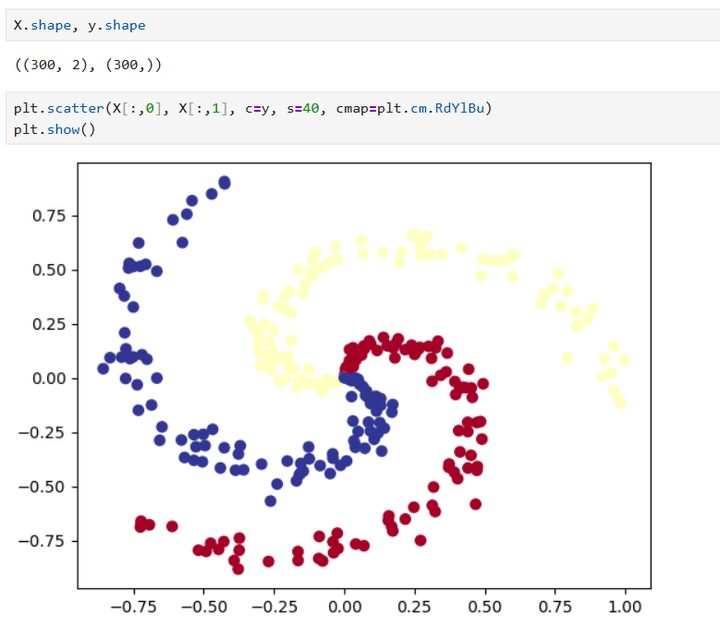
y[ix] = j生成个三分类的数据来训练模型,对于模型来说,多少个分类都是一样训的。
数据大概是长这样子的:
数据现在是numpy,要转成tensor,然后要放到合适的device(放到GPU去),然后还要切分数据为训练集和测试集。
import torch
X = torch.from_numpy(X).type(torch.float)
y = torch.from_numpy(y).type(torch.LongTensor)

X = X.to(device)
y = y.to(device)

from sklearn.model_selection import train_test_split

X_train, X_test, y_train, y_test = train_test_split(X, y, test_size=0.2, random_state=RANDOM_SEED)
模型
from torch import nn

Classification = nn.Sequential(
    nn.Linear(in_features = 2, out_features = 10),
    nn.ReLU(),
    nn.Linear(in_features = 10, out_features = 10),
    nn.ReLU(),
    nn.Linear(in_features = 10, out_features = 3)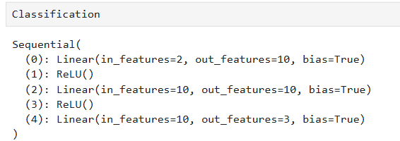
).to(device)这和我们上次做二分类有什么区别,可以说根本没区别,当然如果你仔细看的话,原来二分类的输出是一个logit,然后我们过一个sigmoid,出来分类的概率。这里是多分类,对每一个分类都会有一个logit,所以输出的长度与分类的数目一致,这里是3分类,就设定out_features = 3。这长度为3的logits,依然需要有一个函数给转成这三种分类的概率,这就需要用softmax函数。预测的结果就是概率最大的分类。
损失函数
loss_fn = nn.CrossEntropyLoss()正如我们在二分类里介绍的,分类用交叉熵来计算损失,这里相应地就用了nn.CrossEntropyLoss()函数。
优化器
optimizer = torch.optim.Adam(params = Classification.parameters(), lr = 0.01)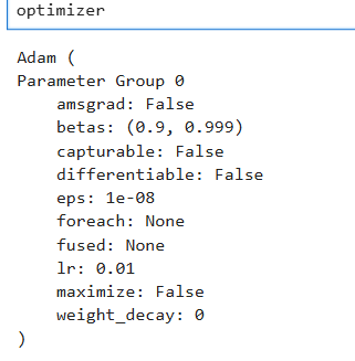
上次我们用随机梯度下降(SGD),这次我们换一个,用Adam,Adam这个方法的基本思路是融合了两种方法:Momentum和AdaGrad。Momentum参照小球在碗中滚动的物理规则进行移动;AdaGrad会记录过去所有梯度的平方和,学习越深入,更新的幅度就越小。Adam通过组合这两个方法的优点,有望实现参数空间的高效搜索。
准确率
from torchmetrics import Accuracy

acc_fn = Accuracy(task="multiclass", num_classes = K).to(device)
acc_fn准确率这个函数和我们做二分类基本一样,差别就在于指定了不同的num_classes参数而已。
训练模型
from timeit import default_timer as timer

start_time = timer()

epochs = 1000

for epoch in range(epochs):
    ## Training
    Classification.train()

    y_logits = Classification(X_train)
    y_pred = torch.softmax(y_logits, dim=1).argmax(dim=1)

    loss = loss_fn(y_logits, y_train)
    acc = acc_fn(y_pred, y_train)

    optimizer.zero_grad()
    loss.backward()
    optimizer.step()

    ## Testing
    Classification.eval()
    with torch.inference_mode():
        test_logits = Classification(X_test)
        test_pred = torch.softmax(test_logits, dim=1).argmax(dim=1)
        test_loss = loss_fn(test_logits, y_test)
        test_acc = acc_fn(test_pred, y_test)

    if epoch % 100 == 0:
        print(f"Epoch: {epoch} | Loss: {loss:.5f}, Accuracy: {acc:.2f} | Test loss: {test_loss:.5f}, Test acc: {test_acc:.2f}")

end_time = timer()和二分类的训练代码基本上是一样的,就是把模型一换,把logits要过一下sigmoid换成softmax而已。
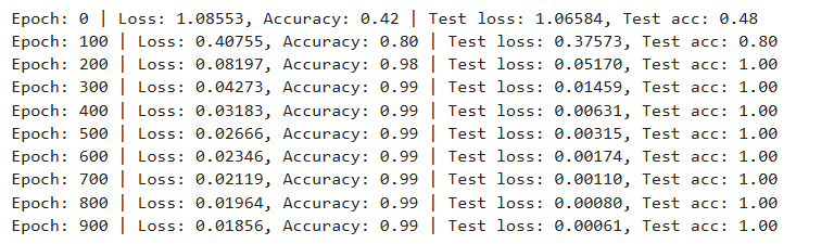
也是很快就收敛了,准确率很高,用时5秒不到。
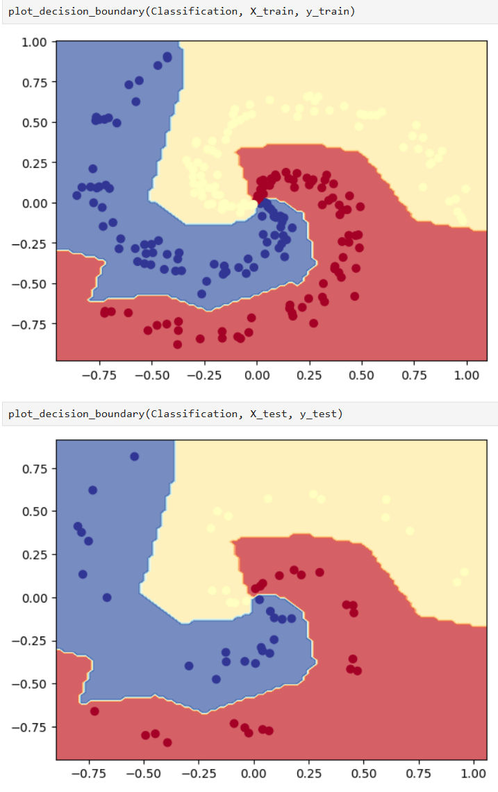
可视化
最后我们把模型在训练集和测试集的决策边界给画一下: